Four Decades of Weather and Climate at the Scottish Association for Marine Science Laboratory on the Dunstaffnage Peninsula in the Scottish West Highlands (1972 to 2014)[1]
Stuart Cunningham, 29th July 2014
“Of mice and men” stated that the arguments about the causes of climate change are settled (in the same way we no longer argue whether the Earth orbits the sun): climate is changing and it is our doing. Practically we need to focus more on the regional impacts of climate change. The OSNAP programme will provide such a focus. This article describes some regional climate – in the west highlands of Scotland, linking this to global climate teleconnections and climate change. We then describe briefly how OSNAP contributes to new knowledge and understanding of how regional climate and wider climate patterns can be linked.
Within the grounds of the SAMS marine laboratory, at Dunstaffnage, the UK Meteorological Office maintains a synoptic weather and climate station. Operating continuously since 1972 we can now investigate climate at this site over four decades. What does it show about the weather and climate in the west highlands of Scotland?
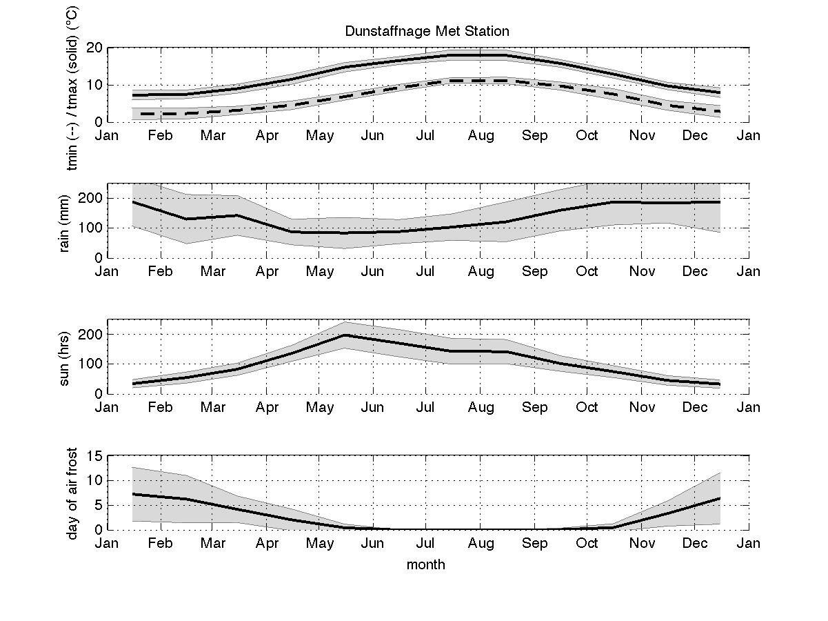
The seasonal cycles of air minimum and maximum temperatures, rainfall, sunshine hours and air-frost days (Figure 1, Table 1) have clearly defined seasonal variations. Our summers are warmest in July and August, but sunniest in May, and notably dry in April, May and June. Overall, we have a wet climate, with an annual average rainfall of 165 cm (5 feet 5 inches for the imperialists amongst you!). But the variability of our weather (and the beauty of our geography) gives a special meaning to fine days. Alastair Reid’s poem “Scotland” perfectly captures the mood swings of the Scottish psyche induced by the Scottish climate (and the Calvanism). For your edification the poem is reproduced at the end of this blog.

Figure 1: Seasonal cycle of monthly mean temperatures (°C, minimum dashed, maximum solid), rainfall (mm), sunshine hours (hrs), days of air-frost (days). The monthly mean temperature is calculated from the average of the mean daily maximum and mean daily minimum temperature i.e. (tmax+tmin)/2.Shaded region is one standard deviation of the monthly mean. The seasonal cycle has been computed from January 1972 to Feb 2014 except for sunshine hours, recorded in two periods: from September 1981 to September 1984 (three years) and from March 1986 to December 2001 (16 years). All the meteorological data analysed here can be downloaded freely from www.metoffice.gov.uk/public/weather/climate-historic/#?tab=climateHistoric.
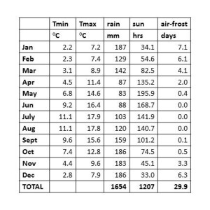
Table 1: The Seasonal Cycle values of monthly mean values of minimum and maximum temperature, (°C) rainfall (mm), sunshine (hours) and number of air-frost days (days).
Climate Trends
We will look now at long-term weather trends of temperatures and rainfall (i.e. the climate). These two variables have quite different patterns of change over four decades, nicely illustrating the complexity of climate.
Temperature
The singular striking aspect of the temperature anomalies at Dunstaffnage (Figure 2) is the pattern of cold anomalies between 1972 and 1995, which are completely reversed to warm anomalies between 1995 and 2010. A linear trend shows a warming of 1.08°C from 1972 to 2014. Shown in the plot are the 95% confidence limits for this trend.
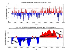
Figure 2: Anomalies of maximum monthly mean air temperature (°C) relative to the seasonal cycle. Top panel shows monthly values and the lower panel 3-month low-pass filtered values. In the lower panel the solid line is the linear trend of the anomalies with 95% confidence intervals. Anomalies of minimum monthly mean air temperature (not shown) are almost identical in monthly pattern and long-term trend. The trend is 1.08°C calculated between 1972 and 2014. This is a trend of 0.26°C/decade.
How does this local temperature change compare to global average temperature changes? Over Earth’s land and ocean surface the average temperature is increasing rapidly: the warming (by linear trend) from 1972 to 2014 is 0.8°C[1]. Most of the observed increase in globally averaged temperature since the mid-twentieth century, is very likely due to a 40% increase in atmospheric carbon dioxide concentration since the pre-industrial era[2]. Dunstaffnage temperatures have risen by 1.08°C, therefore increasing at a rate 26% higher than the global average. Quite possibly this more rapid warming at Dunstaffnage (56.4545° N, 5.4379° W) is linked to the amplification of warming at high latitudes due to decreasing ocean ice cover (amongst a host of other potential feedbacks). Changes in northward heat transport by the oceans and moist atmosphere could also be implicated.
In the last decade global average temperatures have remained constant or decreased slightly, and this is reflected in decreasing temperatures after 2007 at Dunstaffnage (Figure 2). This temperature stand does not mean an end to global warming, but is explained by natural climate variations: large cyclic variations in North Pacific winds[3] have increased heat absorption by the ocean, leading to steady atmospheric temperatures. We have not demonstrated a link between temperatures in Dunstaffnage and atmospheric variability in the Pacific, but it is probable.
Therefore at Dunstaffnage the long-term temperature trend strongly links to the global warming trend and to effects of preferentially increased warming rates at high latitudes. We also see evidence for remote effects of natural cycles of Pacific climate variability in the stand of warm temperature anomalies in the past decade.
Rainfall
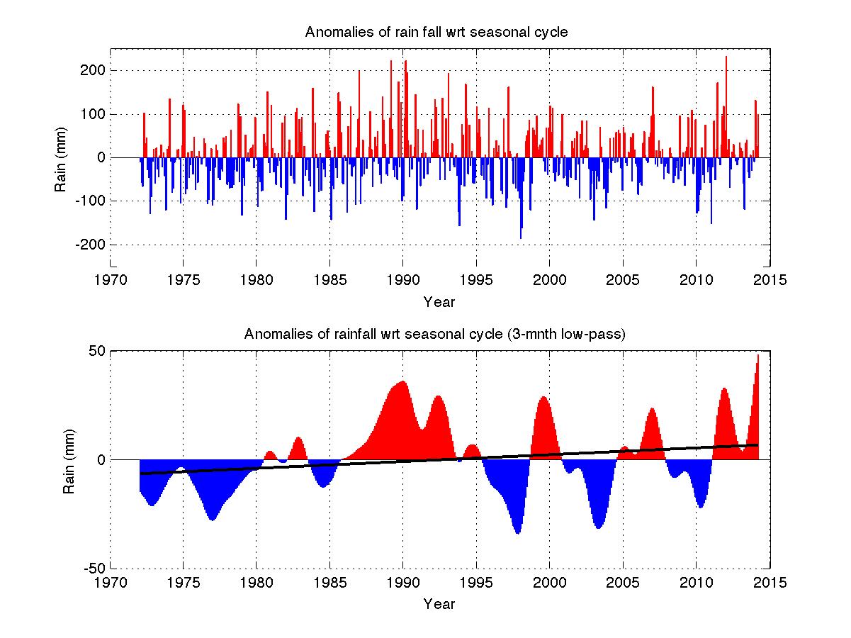
One difficulty with analyzing rainfall data is the large inherent variable. This is readily seen in Figure 2, as the large variation around the mean value in each monthly mean value of rainfall (the grey bars are large): it can be wet or dry at any time of the year with large variations around the seasonal (expected) value.
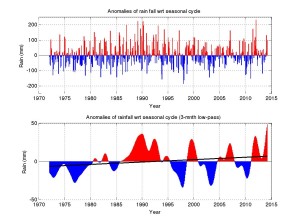
Figure 3: Anomalies of monthly mean rainfall (mm) relative to the seasonal cycle. Top panel shows monthly values and the lower panel 3-month low-pass filtered values. In the lower panel the solid line is the linear trend of the anomalies.
At Dunstaffnage (Figure 3) there is an approximately five-year cycle of wetter and drier periods (particularly since the mid-1990s). The long-term trend from 1972 to 2014 suggests a net increase in annual rainfall of 13 mm (3.1 mm/decade), but statistically this trend is not significant. Our inability to identify long-term trends of observed rainfall is a typical problem for the majority of global rainfall observations.
As an aside, a warming atmosphere holds more water vapor, the content increasing approximately 7% for one degree of warming. The oceans dominate the fresh-water cycle, evaporating 13 million cubic meters of water per second and receiving 12 million cubic meters of water per second in rainfall. The small difference of 1 million cubic meters per second falls as rain over the land. Changes in pattern and amounts of rainfall over the ocean change the oceans’ salinity and thus observations of ocean salinity can tell us about changing precipitation (the ocean rain gauge) – even if trends in rainfall are hard to detect by direct observation over the land.
Although rainfall at Dunstaffnage is an inherently noisy process we can relate it to the main pattern of atmospheric variability in the North Atlantic called the North Atlantic Oscillation (NAO). The atmosphere in the Atlantic has a high pressure centered over the Azores and a low pressure centered over Iceland. The atmospheric pressure difference from the Azores to Iceland strongly controls the direction and strength of weather patterns – the westerly trade winds – that travel from west to east across the Atlantic. When the pressure difference between the Azores and Iceland is larger than normal then storms tend to pass eastward at higher latitudes than normal (north of the UK in extreme cases). This leads typically to wetter (and warmer) conditions over west Scotland. Conversely, for a lower than normal pressure difference, storms track eastward at much lower latitudes, bringing rain to Spain: and dry (and colder) conditions to the west of Scotland.
Comparing rainfall at Dunstaffnage to the North Atlantic Oscillation Index (Figure 4), there is evidently some relationship: often the red (high NAO index/high rainfall) and blue (low NAO index/low rainfall) correspond. While the correspondence is not one-to-one, the variations in the NAO index explain 44% to 57% of the signal in Dunstaffnage rainfall (range is 95% confidence interval). Thus Dunstaffnage experiences rainfall patterns that are strongly related to the latitude at which the west to east moving storms cross the Atlantic.
![Figure 4: (top panel) North Atlantic Oscillation Index. Normalized pressure difference between the Azores high pressure and Icelandic low pressure. Index downloaded on 12th March 2014 from the US National Centre for Environmental Prediction [www.cpc.ncep.noaa.gov/products/precip/CWlink/ENSO/verf/new.nao.shtml]. (bottom panel) Anomalies of rainfall (mm) relative to the seasonal cycle, at Dunstaffnage.](http://www.o-snap.org/wp-content/uploads/2014/07/Figure4_Stuart-300x224.jpg)
Figure 4: (top panel) North Atlantic Oscillation Index. Normalized pressure difference between the Azores high pressure and Icelandic low pressure. Index downloaded on 12th March 2014 from the US National Centre for Environmental Prediction [www.cpc.ncep.noaa.gov/products/precip/CWlink/ENSO/verf/new.nao.shtml]. (bottom panel) Anomalies of rainfall (mm) relative to the seasonal cycle, at Dunstaffnage.
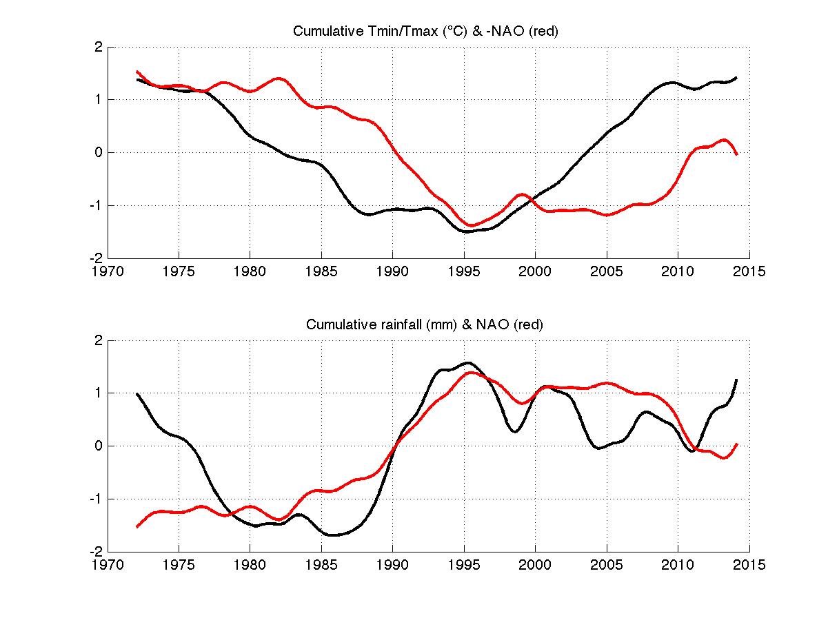
We can extend our comparison of Dunstaffnage rainfall and the atmospheric variability over the Atlantic by thinking how the North Atlantic Oscillation and rainfall changes accumulate over time. That is do drier or wetter patterns persist for many years? To examine this we simply add the rainfall anomalies with time and do the same for the North Atlantic Oscillation Index (Figure 5).
From 1972 to 1986 Dunstaffnage became progressively drier with time (Figure 5). This makes sense looking at Figure 4 where these years have negative rainfall anomalies. Then we enter a wetter period from 1986 to a peak in rainfall accumulation in 1995. Since then Dunstaffnage is trending towards drier conditions, but with the 5-year oscillation evident. The accumulated oscillation index (Figure 5) corresponds closely with the rainfall accumulation. The oscillation index explains 67% to 75% of the signal in accumulated rainfall (at 95% confidence limits). This correspondence between the rainfall and the oscillation index is entirely expected. Hundreds of scientific papers have established links between the oscillation and multiple climate variables: analysis includes both modern data and paleo-climate data, establishing that this pattern has been active for at least 5000 years.

Figure 5: Cumulative addition of Dunstaffnage rainfall (black) and the North Atlantic Oscillation Index all months (red). Both timeseries have been normalized. Accumulating rainfall corresponds to increasing oscillation index.
Discussion
At Dunstaffnage we can link local temperature and rainfall variability to patterns of established climate variability: rainfall to the North Atlantic Oscillation; temperatures to the Pacific Decadal Oscillation. We can also identify the global warming temperature trend at Dunstaffnage and find that it is larger than the global average temperature rise: we suggest this is related to more rapid warming that happens at higher latitudes.
Regrettably, I have falsified the title of this article “‘Dinnae expect onything an ye’ll no be disappointed”, by demonstrating that by examining data around the globe can tell us with some confidence what to expect, both for long-term temperature trends and for rainfall trends.
So can we better understand these global to regional teleconnections in weather and climate patterns? The Overturning in the subpolar North Atlantic Programme is measuring the circulation in the subpolar North Atlantic because there is mounting evidence that knowing the circulation in this region leads to improved decadal climate prediction. Both modelling and observations studies link temperatures and currents in the subpolar gyre to tropical storm and hurricane frequency, rainfall in the Sahel, Amazon, western Europe and parts of the US, on wind strength and on marine ecosystems.
Thus the contribution of OSNAP to this much wider climate forecast problem is to generate new knowledge and understanding of the subpolar gyre by measuring the circulation and fluxes of heat and fresh water from Newfoundland to Greenland to Scotland. This continent-to-continent observing system will enable the relationships between circulation, ocean and atmosphere exchanges and climate impacts, for the first time, to be examined with a purposefully designed observing system.
Progress is oftentimes by small steps, but occasionally extraordinary efforts to take leap forward need to be taken.
Scotland
It was a day peculiar to this piece of the planet,
when larks rose on long thin strings of singing
and the air shifted with the shimmer of actual angels.
Greenness entered the body. The grasses
shivered with presences, and sunlight
stayed like a halo on hair and heather and hills.
Walking into town, I saw, in a radiant raincoat,
the woman from the fish-shop. ‘What a day it is!’
cried I, like a sunstruck madman.
And what did she have to say for it?
Her brow grew bleak, her ancestors raged in their graves
as she spoke with their ancient misery:
‘We’ll pay for it, we’ll pay for it, we’ll pay for it.’
Alastair Reid
View as PDF
[1] This article was written as a contribution to the 130th year of SAMS and its parent labs and also forthe centenary of Sir John Murray KCB FRS FRSE FRSGS (3 March 1841 – 16 March 1914) a pioneering Scottish oceanographer, marine biologist and limnologist.
[2] CRUTEM4 from the Climatic Research Unit (University of East Anglia).
[3] These results quoted directly from IPCC AR5, Summary for policy makers. See ahttp://www.ipcc.ch/WG1AR5_SPM_FINAL.pdf
[4] Cool phase of the Pacific Decadal Oscillation


![Figure 4: (top panel) North Atlantic Oscillation Index. Normalized pressure difference between the Azores high pressure and Icelandic low pressure. Index downloaded on 12th March 2014 from the US National Centre for Environmental Prediction [www.cpc.ncep.noaa.gov/products/precip/CWlink/ENSO/verf/new.nao.shtml]. (bottom panel) Anomalies of rainfall (mm) relative to the seasonal cycle, at Dunstaffnage.](http://www.o-snap.org/wp-content/uploads/2014/07/Figure4_Stuart.jpg)
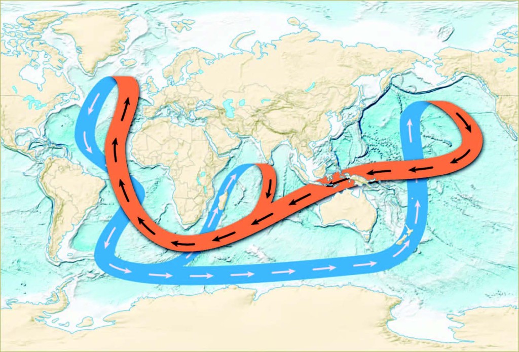 g circulation” refers to the generally northward flow of warm and salty water in the upper ocean, and the southward return of colder, fresher water deeper down. The system of ocean currents that makes up the overturning circulation has been efficiently depicted in various schematic diagrams and is often referred to as the Great Ocean Conveyor. It is important however not to interpret this schematic as exactly representative of the deep and shallow currents in the North Atlantic. A more realistic view is shown by the second diagram below, but even this suggests overly smooth and well-behaved current pathways.
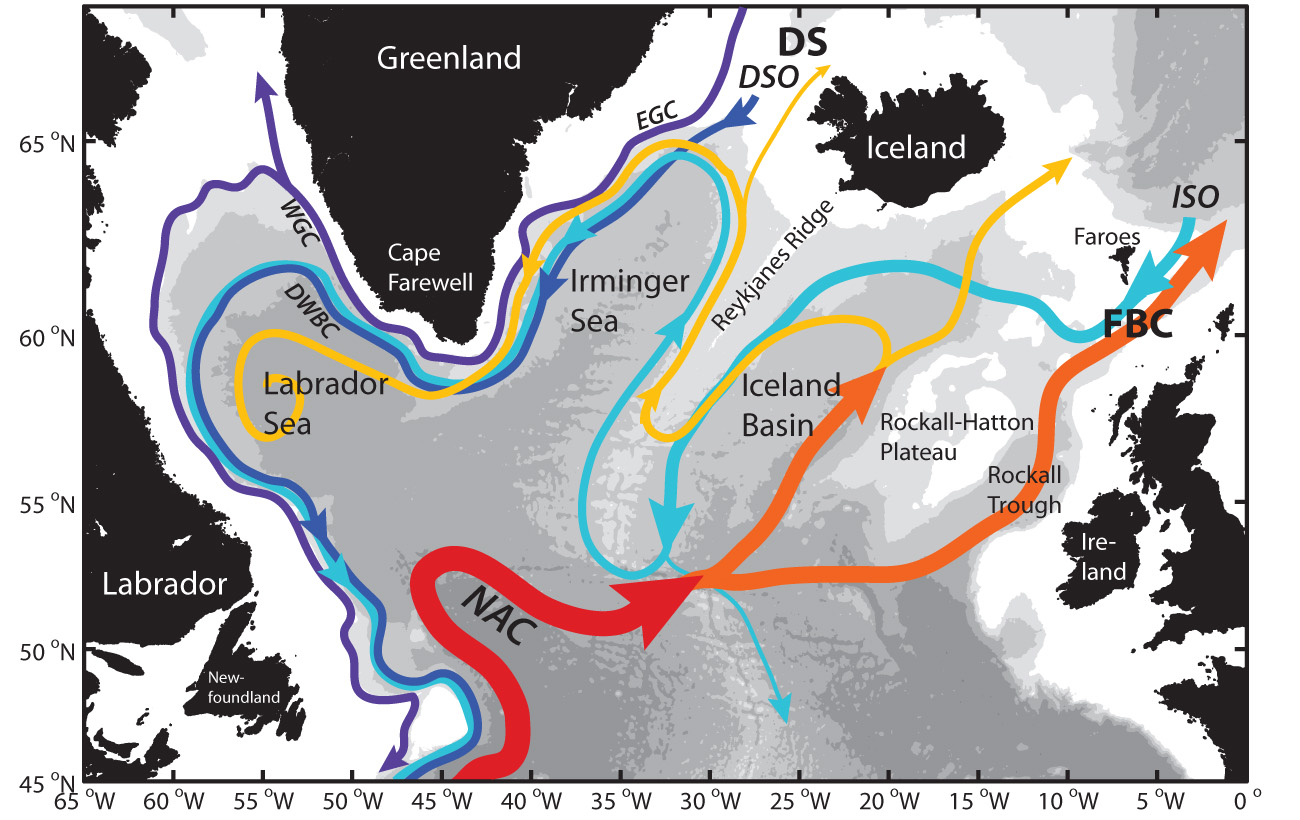
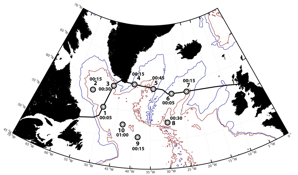 day, the beacons emit an 80-second tone at about 260 Hz. Then we release floats from the research vessel at various locations where we know the currents are located. The floats have just the right weight (measured within 1 gram) to sink and drift 200 meters above the sea floor. Attached to each float is an underwater microphone, called a hydrophone. The floats will listen for the beacons and record the time that they hear the sound signals. They will do this for two years, then drop some weight so they can rise to the sea surface and transmit the recorded information to us via satellite. Knowing the time the signal was sent, and each time it reached the float and the speed of sound in seawater, we can figure out the distance between the float and each sound beacon. As long as the float hears signals from at least two beacons, we can figure out where the float was every day. By connecting the dots from day to day, we end up with the float’s trajectory and the path of the water it was drifting with. With many floats, we can generate a description of where the currents go most frequently. We can also observe meanders and eddies in the currents.