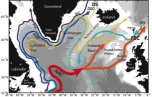
Over the past several decades, oceanographers have constructed maps of the deep currents in the North Atlantic by piecing together measurements of currents and water properties from widely separated locations at different times. An example is shown in Figure 1. Such diagrams are beautiful in their simplicity and valuable for communicating the importance of northward-flowing warm and southward-flowing cold currents that together transport vast amounts of heat from the equatorial to polar regions.
Figure 1: Schematic diagram of the major currents thought to be responsible for northward heat transport in the subpolar North Atlantic.
While useful as a summary of buy lasix canada subpolar North Atlantic overturning circulation, we need to remind ourselves that such ‘plumbing’ diagrams, if taken too literally, can give the false impression that there is very little connection between the boundaries of the ocean basin and the interior. Acoustically tracked underwater drifting buoys (called RAFOS floats) are being deployed in the deep boundary currents of the subpolar North Atlantic as part of OSNAP to investigate this connection (see previous posts for more details about the RAFOS float program in OSNAP at http://www.o-snap.org/water-goes-here-water-goes-there/ and http://www.o-snap.org/glass-floats-embark-on-a-2-year-mission-at-sea/). This Lagrangian approach to measuring ocean currents, whereby freely drifting floats reveal deep current pathways by drifting with the water (in contrast to the Eulerian approach, whereby sensors fixed in one position measure current speed and direction over a period of time) is ideal for mapping out current pathways over a large area, and with repeated deployments, we can determine how those pathways are changing in time.
Animations of the observed changes in the physical properties of the North Atlantic can really help us to understand their geographical distribution and their evolution over time. We’ve created a series of animations of different properties, and here show a few to give you a flavour of the insight they provide. You can see more on our YouTube Channel.
The North Atlantic Ocean anomaly animations are based on a reanalysis of historical temperature and salinity data by Dr Doug Smith at the UK Met Office, where the sparse observations are mapped using model covariances from a Hadley Centre model (Smith and Murphy, 2007). The plots are made by Dr Vassil Roussenov and the videos by Dr Andy Heath, and Prof. Ric Williams (all from the University of Liverpool) is the lead investigator; this work was supported by the UK Natural Environment Research Council.
This is an animation of annual anomalies of ocean heat content (10^8Jm^-2) over the North Atlantic, where red is warm and blue is cool. The annual anomalies are defined relative to a time average from 1950 to 2010, and are evaluated for the full ocean depth. The animations reveal the strong interannual and decadal variability. There are often different responses occurring in the subtropical and subpolar gyres (Williams et al., 2014), as well as occasions when thermal anomalies appear to pass from one gyre to the other. At the same time, there is an overall warming trend over this 60 year period, represented by the anomalies becoming warmer over the last decade. The different decadal responses are emphasized by the pictures of the time-averaged thermal anomalies for 1950-1970, 1980-2000 and 2000-2010.
The mechanisms forming these ocean heat content anomalies involve the imprint of changes in wind forcing, physical transport and redistribution of heat within the basin, and local and far field changes in air-sea heat fluxes. The dominant mechanisms probably vary with the location and timescale of interest.
Sea surface height varies for a range of reasons. Atmospheric forcing induces waves and even storm surges, while gravitational effects of the Moon and Sun induce the predictable tidal undulations in sea level. The sea level also responds to the heating and cooling of the ocean, sea level increasing from the water column expanding when the water warms or freshens. The sea level likewise increases from the addition of mass from more water added to the global ocean from river runoff and melting of ice on land.
The animation shows the annual sea surface height anomalies in sea level (mm) in the North Atlantic calculated from how the water column expands when there is warmer or fresher water. The sea level varies by -50 mm (blue) to +50 mm (red) due to these volume changes. The animation reveals a similar response to ocean heat content change, regions of heat gain associated with a higher sea level (red) versus regions of heat loss associated with a lower sea level (blue). Again there is strong decadal variability for the ocean gyres, as well as a background rise in sea level over the entire record.
The mechanisms forming these sea surface height anomalies involves the imprint of changes in wind forcing, physical transport and redistribution of heat and freshwater within the basin, and local and far field changes in air-sea heat and freshwater fluxes. The dominant mechanisms probably vary with the location and timescale of interest, although much of the local variability is likely to involve a redistribution of warmer and lighter waters.
Sea surface temperature varies due to solar heating and air-sea exchange of heat, as well as due to transport of warm waters and mixing with cooler, deeper waters. The animation shows the annual anomalies in sea surface temperature (C) in the North Atlantic, varying from -1.5C (blue) to +1.5C (red). The animation is broadly similar to the ocean heat content change, regions of higher sea surface temperature generally coinciding with greater ocean heat content, although there are detailed differences, particularly in the subtropical latitudes. Again there is strong decadal variability for the ocean gyres, as well as a recent surface warming for 2000 to 2010.
The sea surface temperature (SST) anomalies are generally viewed as being driven by anomalies in air-sea fluxes on interannual timescales (greater heat input from the atmosphere leads to warmer SST), but might feedback back and determine the air-sea fluxes on decadal or longer timescales (a warmer SST leads to a greater loss of heat from the ocean to the atmosphere). There is also a physical transport of the SST anomalies on all timescales.
Many of the OSNAP blog stories we’ve posted so far give a flavour of the exciting array we have deployed in the subpolar North Atlantic, and the process by which we have achieved this. With a fleet of 4 ships and a diverse team of scientists and engineers, over the course of the 2014 summer we put in place our measuring system that will tell us so much about the circulation of the region. Many of our instruments lie unattended and uncommunicative in the darkness of the deep ocean until we haul them out of the depths and back into fresh air one or two years later. We harvest the data as soon as they come back onboard and the long process of turning a large set of numbers into information about the changing ocean begins.
So you might think that now the instruments are in the water we can take a break, do something else, and just wait for the next cruises to come along. Or you might guess the truth, which something rather different. The detailed planning for next years’ cruises has already started, and work on data collected during the array deployment cruises, and from instruments that are communicative while they roam the ocean, is well underway.
“AMOC, consisting of a northward flow of warm surface waters and a southward flow of cold deep waters, is the leading mechanism for heat transport and carbon sequestration in the Atlantic Ocean,” said Macdonald and Wunsch in 1996.
As the key component of global meridional overturning circulation, Atlantic Meridional Overturning Circulation (AMOC) plays a significant role in modulating the global climate system, which has drawn continuous attention from oceanographers for decades. However, increasing knowledge on the AMOC has not clarified its nature, but led us to more confusion.
Studies on the mechanism of AMOC can date back to 1950s, when AMOC was viewed as a source/sink-driven overturning cell and often simplified as a conveyor belt for exporting the deep water formed in the high latitude of the North Atlantic to the low latitude and South Atlantic. Variability of the AMOC was supposed to be controlled by either the source, i.e., the production of deep water, or the sink, i.e., the return of deep ocean water to the surface. This simple framework has been dominating our society for decades.
However, this traditional view has been challenged lately by a number of studies. Dr. Jian Zhao, who just completed his doctorate from University of Miami, suggested seasonal cycle of AMOC, and a large part of AMOC interannual variability at 26.5°N, are controlled mainly by wind forcing. Jiayan Yang, a PI from Woods Hole Oceanographic Institution, says,“Recent work shines light on that it is the wind stress not the buoyancy flux that is the leading mechanism for AMOC variability from seasonal to interannual, even decadal time scales.”
As the swift pace of the OSNAP field season has wound down, we have been gathering profiles of the students and postdocs who are working on OSNAP projects. So, with this post I would like to welcome those young oceanographers: Till Baumann (GEOMAR, Helmholtz Centre for Ocean Research), Elizabeth Comer (National Oceanography Centre and University of Southampton), and Nick Foukal and Sijia Zou (Duke University) are graduate students working on OSNAP projects and Loïc Houpert (Scottish Association for Marine Sciences) and Neill Mackay (National Oceanography Centre) are postdocs. See: http://www.o-snap.org/partners/students-postdocs/ for more information about these oceanographers and their projects. As with almost all other large scale ocean observational programs, OSNAP was designed by those of us who have been oceanographers for a number of years, if for no other reason than the planning itself can take a number of years. Continue reading →
“Pay out the wire slowly and keep it tense in the water, okay?”
“Got it!”
“Okay, go ahead.”
It was another foggy and calm morning in the Subpolar Atlantic onboard the R/V Knorr. John Kemp, the mooring group leader, was teaching Chun Zhou, a physical oceanography PhD student from China, how to drive the winch to lay the mooring wire rope into the water. Almost two months have passed since the end of that cruise. However, some people may still remember Dalei Song, Xiaoman Yang, and Chun Zhou, the three Chinese guys on board who were there representing the Ocean University of China (OUC) and making the university’s first move in cooperation with partners as one of the members of OSNAP.
OSNAP is a US-led international collaborative project designed to provide a continuous record of the full-water column, trans-basin fluxes of heat, mass and freshwater in the subpolar North Atlantic using a network composed of moorings, ship-based hydrographic sections, RAFOS floats and gliders. As planned by the principal investigators, the objective for Cruise #Kn221-03 was to deploy moorings, carry out several high-resolution CTD sections, and deploy dozens of RAFOS floats. Taking into consideration the OUC participants’ experience with mooring operation, Dr. Bob Pickart, the chief scientist of this cruise, assigned them to John, who led a small group comprised of the best hands in mooring operation. Continue reading →
Late last month I attended a symposium in London celebrating the tenth anniversary of the UK-US RAPID array at 26°N in the subtropical North Atlantic. All assembled agreed that this first continuous measure of the ocean’s meridional overturning circulation has produced a dramatic shift in our understanding of the large scale ocean circulation in the North Atlantic. Those of us working on the OSNAP project understand all too well that with this dramatic shift RAPID has set a high bar for success. So, to all RAPID PIs, let me offer a congratulatory note on behalf of all OSNAP PIs on this milestone. Well done.
For those of us involved in these large scale ocean observing programs, we have little to no doubt as to their benefit to our science in the short run, and to society in the longer run. But these observations come at a price that is sizable to most any funding agency. This price tag, coupled with the dawning realization that we will need to measure for years and years in order to discern long term trends of the overturning and its attendant heat, carbon and freshwater fluxes, should give us pause. This message more or less was delivered to those assembled in London in the closing remarks given by Professor Duncan Wingham, Chief Executive of the UK National Environmental Research Council (NERC). Professor Wingham noted the irony of an Environmental Research Council funding ships to crisscross the ocean all the while burning (lots of) fossil fuels. It is though the cost of business and oceanographers can hardly be held responsible for the rising cost of fuel over this past decade. And yet, all of us understand that with anything the price must be commensurate with the value added. While we as oceanographers are convinced of the value, I think it is safe to say that outside of our community it may not be so patently obvious. Continue reading →
The largest water fall in the world is an underwater waterfall. Its just northwest of Iceland, and it begins with water spilling over an underwater ledge between Iceland and Greenland, the Denmark Strait.
Hurtling down this water fall are cyclones of water, 1,500 meters high.
Bob Pickart was the first to measure the cyclones in 2008. He measured them by accident: They spent a year whacking into 4 stationary vertical strings of instruments that he had placed in the ocean. These moorings were at the bottom of the waterfall, a checkpoint to see what it did after it spilled off. When he went to collect the data— a year’s worth —he found that it was garbled. Instead of examining a vertical slice of the ocean, the instruments had been repeatedly pushed over at an angle. What emerged from the mess was a picture of a tornado-like column of water, rushing past about once every two days.
This is how they form: As dense water moves over the Denmark Strait, it sinks. (It does this over the course of 100 of kilometers —though taller than Niagra falls, this under water water fall is not a steep waterfall.) As that water sinks, it starts to spin —kind of in the same way that a figure buy hydrocodone online skater hugs her arms to her chest to spin faster. The result: a towering, whirling column of water.
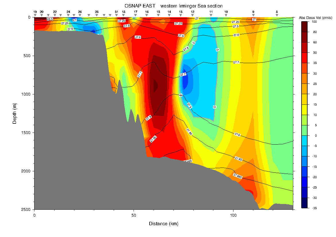
If you measure its velocity, it looks like this:
The red part is coming at you at 80 cm/s, the blue part is going into the screen at 30 cm/s (slower, because the whole thing is also moving southward.)
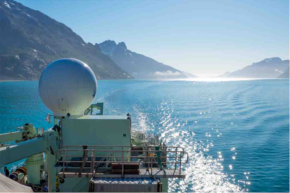
“Greenland is great because it has complex boundary currents,” explains Bob Pickart. That’s why, in the course of our trip, we’ve spent a lot of time hanging out around Greenland: to study the currents that snake around the sloping ocean floor near it. Scientists on board the Knorr are accomplishing this with round-the-clock deployments of various instruments.
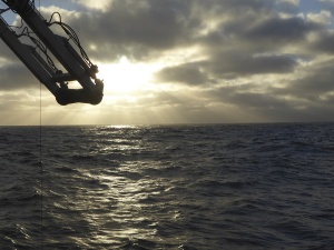
But Greenland is also great because it is very scenic. After days of hovering to the east of Greenland, the science crew took the day off as we steamed through the Prince Christian Sound.
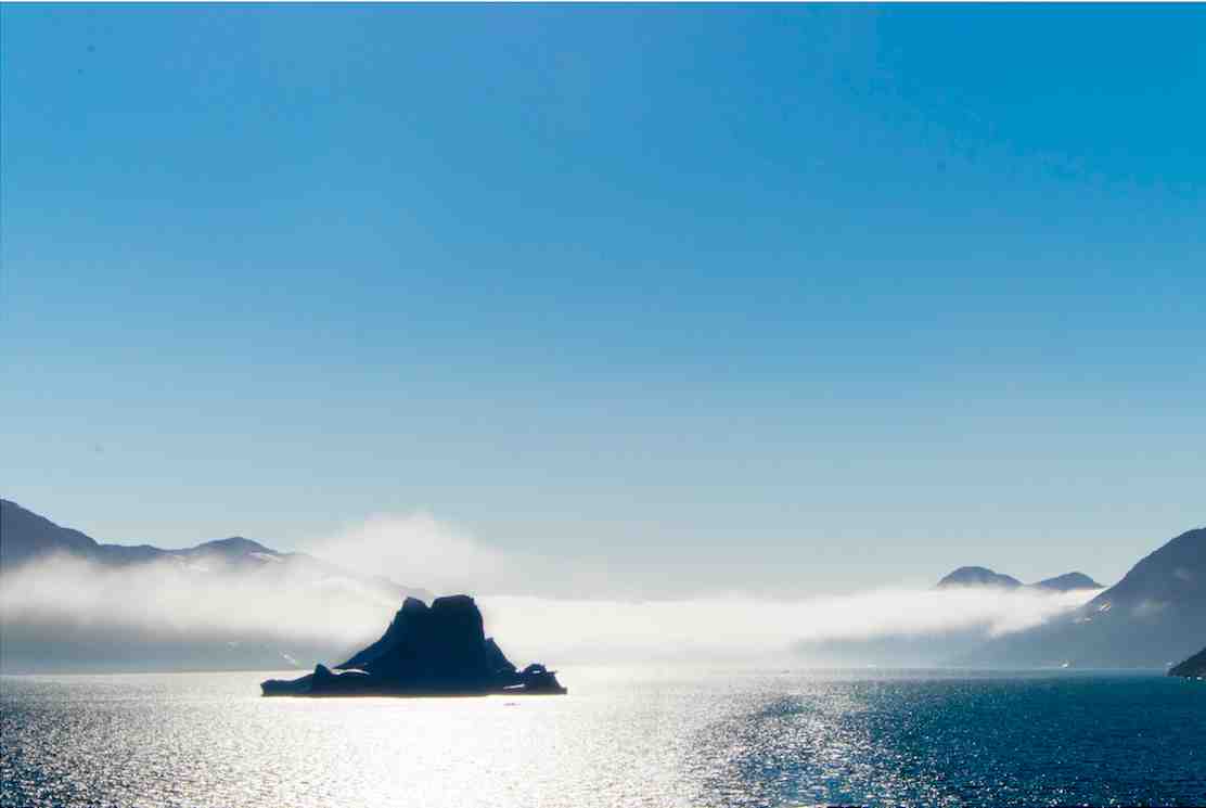
A narrow channel called the Prince Christian Sound splits the very southern bit of Greenland from the rest of the remote land mass. For most of the year, it is clogged with pack ice. For now, its clear —save for icebergs, and little chunks of ice called “growlers” — allowing water, and a few ships, to flow through. The water in this channel is a mere trickle compared to the North Atlantic, so we’re not here to study it, just to use it as a throughway. (It would be an equally long trip to travel around the tip of the country.)
As our chief scientist Bob Pickart says, we’re out here on the ocean to build a “picket fence.” Practically though, the pickets in this fence – moorings – are needle-thin on the scale of the ocean. We only have about 40 “needles” (deployed by this leg of OSNAP and others) to span the entire North Atlantic and the flow we’re measuring is about 15 times stronger than all the rivers in the world combined. This is a tall task, so how do we do it?
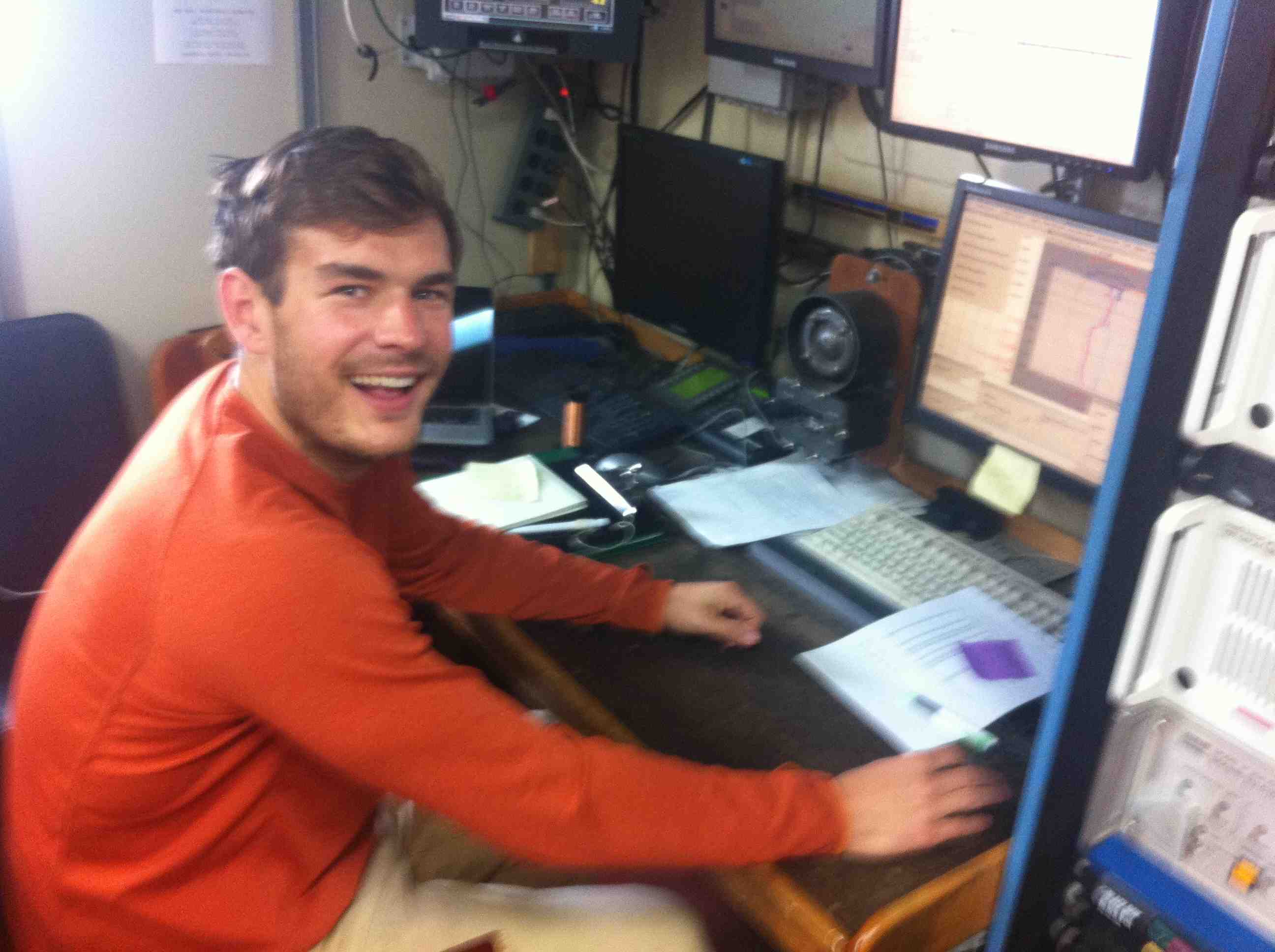
Nick Foukal at work at the CTD watch station.
The key is the ocean’s density, which is a function of the water’s temperature, salinity and pressure (pressure increases as one goes deeper). As luck would have it, many of the instruments we are deploying on this cruise measure those three variables. And from those data we can construct a map of density across the OSNAP line.
For the most part, the densest water in the ocean is near the bottom. Heavy things sink: that much is fairly intuitive. But there are also areas where the density contours (also called isopycnals) are sloped, and these are locations where the flow tends to be strongest. Dense water wants to flow under less dense water, but due to the rotation of our Earth – we’re looking at a huge distance, almost 10% of the circumference of the planet – instead of that dense water flowing toward the less dense water, it often flows 90° to the right of where it should (in the southern hemisphere the water flows 90° to the left). This is what oceanographers call ‘geostrophic flow’, and most of the ocean obeys the rules of geostrophic flow (areas that don’t always obey geostrophy include coastal regions, the bottom and the very surface). It’s like attempting to push someone overboard and the person ending up on the deck next to you – not exactly intuitive. If that’s hard to understand, you’re not alone: as I enter my fourth year of graduate school in oceanography, I’m still trying to come to grips with this phenomenon… that is the geostrophy one, not the man overboard experiment – I’m pretty sure I know how that one would end up.
 of scientists and engineers, over the course of the 2014 summer we put in place our measuring system that will tell us so much about the circulation of the region. Many of our instruments lie unattended and uncommunicative in the darkness of the deep ocean until we haul them out of the depths and back into fresh air one or two years later. We harvest the data as soon as they come back onboard and the long process of turning a large set of numbers into information about the changing ocean begins.