Category Archives: News

by Laura de Steur

OSNAP 9: R/V Pelagia (EAST Leg 2)

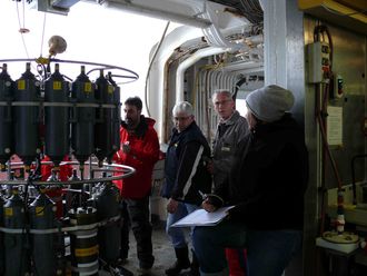
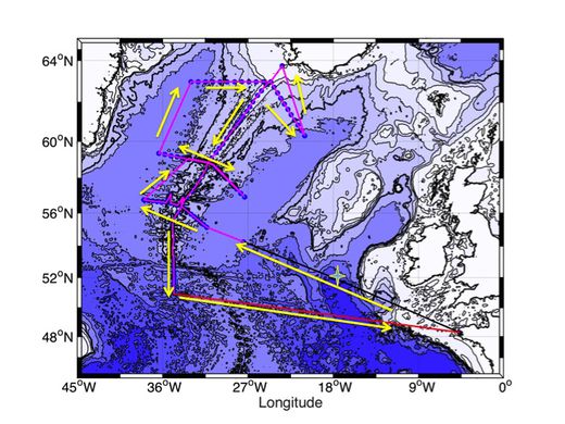
As mentioned before, the recovery of the first moorings on this cruise was very successful: all but one instrument on the 5 Dutch moorings in the Irminger Current had recorded data for one whole year. The large data return of ocean temperature, salinity and velocity at 15 minutes to one hour intervals at selected depths between 100 m and 2900 m depth allows us to investigate the northward flowing Irminger Current. Earlier estimates were derived from summer data (shipboard data) only. Now we can quantify the total volume and heat transport of the Irminger Current based on these continuous measurements, address seasonality, and investigate variability in relation to e.g. atmospheric patterns. After retrieving our data, the instruments have been serviced, batteries replaced, and the moorings are deployed again on the Reykjanes Ridge – ready to collect another year of data. We are now working our way westward in the Irminger Sea and have reached the English moorings in the Deep Western Boundary Current, the cold and dense current flowing southward. Cross our fingers for another few days with good mooring recoveries!

by Laura de Steur

OSNAP 9: R/V Pelagia (EAST Leg 2)

Since we arrived at the moorings sites in the northward flowing Irminger Current on the Reykjanes Ridge, we have been working around the clock. With all 5 moorings recovered in two days, and needing to deploy those again soon, the days seemed too short and time flew by. We will show and tell more soon about these mooring recoveries (YES, with a lot of excellent data to work on for at least a little while). As we needed a couple of days to prepare our instruments again to redeploy the moorings for another year we did 20 full-depth CTD stations (so high ordertramadol resolution) whilst steaming back towards the start of the mooring line on the top of the ridge. This short video illustrates that…

There are a number of OSNAP events coming up over the course of the next few months. You can follow the cruise blogs here: http://www.o-snap.org/news-events/blog/. Please feel free to send any questions to sarah.clem@duke.edu.

• June 5th – July 10th: RREX cruise aboard R/V Thassala across Reykjanes Ridge.
• June 8th – July 7th OSNAP 8 cruise aboard the R/V Pelagia (Leg 1)  to service Iceland Basin and the Rockall Channel moorings and to deploy RAFOS buy prednisone online floats over the slopes east of the MAR ridge crest.
• July 8th – July 29th OSNAP 9 cruise aboard the R/V Pelagia (Leg 9)
• July 21st – A half-day OSNAP meeting (9:00 am-12:00 pm) will be held in Bristol, UK prior to the RAPID-US AMOC International Science Meeting.

Also, Canadian scientists aboard the CCGS Hudson finished their annual Labrador Sea survey recovering three OSNAP moorings and deploying new moorings along the Labrador slope at 53ºN.

By Chris Wilson and Neill Mackay

Figure 1: A schematic of the OSNAP array. (Credit: Penny Holliday).

The OSNAP array (Figure 1) will sample what is effectively a two-dimensional ‘slice’ of the ocean for several years at high spatial and temporal frequency. Of course, as shown in Figure 1, the ocean circulation is three-dimensional, and it varies in time. It contains a range of dynamical scales, from millimeters to millennia. As well as understanding the observations in the OSNAP array ‘slice’, our aim is to build a more complete picture of the circulation and to be able to make statistically robust statements about its variability in a changing climate. For example, is a change measured by the array over, say, a few months representative of a larger branch of the North Atlantic circulation, is it a response to external forcing or is it simply due to local intrinsic nonlinear variability?

Continue reading →

by Penny Holliday

The OSNAP array is designed to meet our scientific objectives by making the most of existing measurements as well as collecting new observations. The eastern part of the array lies along part of a repeat hydrographic section called the “Extended Ellett Line”, or EEL for short. The EEL crosses the deep ocean between Iceland and Scotland, measuring the warm Atlantic water that flows from the subpolar region into the Nordic Seas and eventually the Arctic. The programme has been in place now for an amazing 40 years (1975-2015), making it a rare thing: a multi-decadal time series of high quality, deep ocean measurements. Holliday and Cunningham (2013) (http://www.tos.org/oceanography/archive/26-2_holliday.html) gives a full account of the history and achievements of the programme.

The EEL began in 1975 as a short hydrographic section across the Rockall Trough that was carried out several times a year, though rarely in the winter when the weather is hideous and waves are too big for research vessels to work (see Holliday et al 2006, http://onlinelibrary.wiley.com/doi/10.1029/2005GL025238/abstract to find out how alarming winter research cruises can be). Four decades of observations show that the top layer of the ocean (here around 0-800m) has warmed and there is a lot of shorter timescale variability (Figure 1). The salinity time series shows that there are also periods of highs and lows in salinity, each a few years in length. Look closely and you will see that the most recent years (since about 2010) have been slightly cooler and fresher than the mid 2000s, though values are still high compared to the first half of the time series. A new study of ocean heat content using Argo float data (Roemmich et al, 2015, http://www.nature.com/nclimate/journal/v5/n3/full/nclimate2513.html) confirms that the upper layer (0-2000m) of the northern buy viagra online subpolar North Atlantic has cooled since 2006 while the global ocean heat content has continued to rise. The reason for the patchiness of changes in ocean heat (and freshwater) content is ocean circulation, and OSNAP will bring us new understanding of the processes that underpin the changes we observe.

Continue reading →

by Nick Foukal

For the past 15 years, the slope of the global-mean surface air temperature (GMST) record has plateaued, a change that almost none of the IPCC global climate models (GCMs) predicted. More recently, a couple of papers have come out pointing to the North Atlantic (specifically the subpolar gyre) as the primary location for the missing heat of our climate system [Chen and Tung, 2014; Drijfhout et al., 2014]. The argument goes that because anthropogenic forcing (i.e. greenhouse gases) has increased over this period, yet GMST has not continued to increase, then the oceans must be storing the excess buy diflucan online heat. The North Atlantic is one of the few ‘deep water formation’ sites, thus it is a good candidate to absorb the heat. But let’s quickly review some background information and then the evidence for the North Atlantic.

Background

– Although almost none of the IPCC models predicted this slowdown in global warming, the SAT has never deviated outside of the ensemble range of the models, and 2014 (the warmest year on record) falls directly on the slope of warming from 1970-2000. Some climate scientists thus consider the hiatus as nothing more than noise about a warming trend, while others view it as proof that our GCMs are flawed. Continue reading →

By Amy Bower and Heather Furey

During the summer of 2014, the first setting of 40 deep acoustically-tracked RAFOS floats was made along the OSNAP line (see Mysteries of the Deep Subpolar North Atlantic). Most of these floats were programmed in advance to stay submerged for two years, all the time drifting passively with the deep currents. However, a few floats were programmed for only 180 days so that we could determine how the sound sources are working and how well we were able to adjust the floats’ weight so that they drift just about 100-200 m above the sea floor. Believe it or not, a half year has already passed since the floats were deployed, and the three scheduled to surface after that time have done so over the past few months.

The data collected by these floats indicate that the sound sources all seem to be working properly. The floats were not able to hear the sound sources continuously because of the extremely rough topography of the Reykjanes Ridge, the submarine mountain range that extends southwestward from Iceland forming part of the mid-Atlantic ridge system. Sometimes the floats drift behind underwater mountains that prevent the acoustic signals emitted by the sound sources from reaching the float. This can lead to a short gap in our knowledge of where the float was during that time. This is completely expected and we can usually interpolate the float position during the time it is “invisible”.

Continue reading →

by David Marshall

Fundamental questions we would like to answer in OSNAP are how changes in wind, thermal and freshwater forcing over the subpolar Atlantic modify the Atlantic Meridional Overturning Circulation (AMOC) at lower latitudes and on what time scales? These teleconnections are hard to unravel due to the complexities of the three-dimensional ocean circulation.

A conventional approach to addressing such questions to take a state-of-the-art ocean circulation model and modify the surface forcing in a large number different locations at different times in the past. The problem with this approach is that there are literally thousands of wind, thermal and freshwater forcing anomalies that we need to consider, each requiring a separate model integration.

An alternative approach, which we have used to interpret the AMOC time series at 26.5^oN from the RAPID-MOCHA array, is to use an adjoint model (Pillar et al., 2015). The basic idea of an adjoint model is both simple and surprisingly subtle. Rather than run the model forwards in time, we run it backwards. In a conventional forward model, you perturb the initial conditions, for example, the wind forcing at some time in the past, and see how the three-dimensional circulation evolves differently at all times in the future. In an adjoint model, we purturb a single output, for example the AMOC at 26.5^oN, and by run the model backwards to see how that output is sensitive to all forcing anomalies in the past.

Continue reading →