Category Archives: News

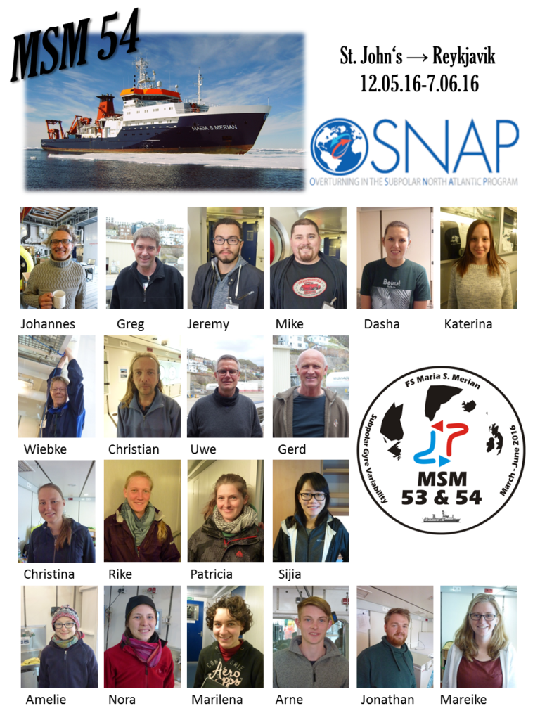
by Nora Fried and Patricia Handmann

Today this blog is focusing on one of the central Instruments of almost all oceanographic cruises: the CTD – Conductivity-Temperature-Depth sensor. One of the interests in oceanography is on the physical, chemical and biological properties of seawater. Most oft the work on board is accumulated around the CTD schedule. The CTD we use on this cruise went on around 70 dives until now, but what exactly is a CTD?

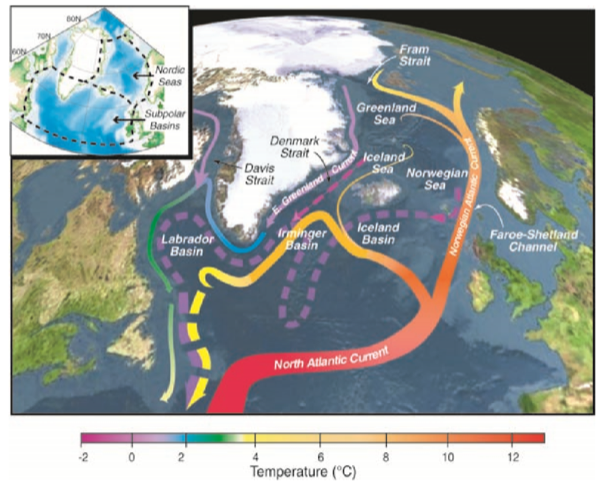
A CTD-rosette consists of a metal cage with a centrally installed sensor pack – the CTD. These sensors are measuring conductivity, temperature and pressure in real time being consistently pumped while passing through the water column. Salinity can be computed from conductivity, temperature and pressure. The maximum depth this instrument can resist is around 6000m. Since our cruise is passing through Labrador and Irminger Sea our deepest station until now is around 3800m deep.

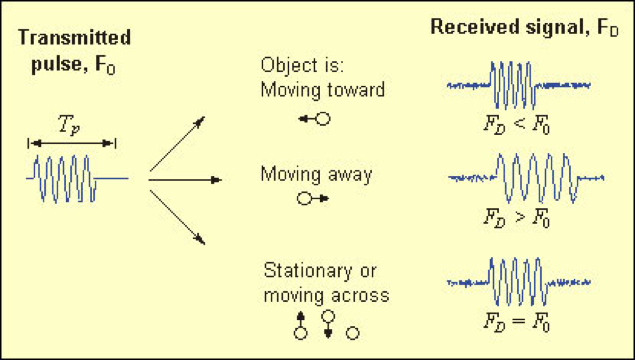
Furthermore there are up to 24 Nisken water sampler bottles, which can hold up to 12 liter of seawater and bring them up to the surface. Additionally to the CTD sensors and the water sampler bottles we installed some more sensors on the CTD this cruise: we measure oxygen concentration, fluorescence, velocity of the surrounding water, distance to the bottom light penetration depth and the turbidity.

The whole CTD-rosette is mounted on a wire, which is connected to the vessels winch system to veer out the instrument into the water and heave it back to the deck. The wire is a cable at the same time and makes real time data transmission from the sensors to a computer on board possible. So temperature, salinity and pressure of the surroundings can be monitored the whole time.

Once a CTD Station is reached and the instrument is prepared the rosette can be deployed. Before deploying the bridge has to approve of the action, then the winch driver is informed by the CTD watch that the instrument can be deployed. The instrument is then veered out with a velocity of around one meter per second – so the CTD watch has to observe the altimeter and all the other instruments the whole time in order not to hit the ground.

Due to different properties of seawater in different depths, density oft the surrounding water is changing and the CTD is drifting with the currents – the pressure is different to the length oft the veered out rope. Therefore the winch is stopped at a depth of 10 to 15 meters to the ground in order not to hit the ground with the sensors. Once the instrument has reached the full depth the first water sampler is closed and the instrument is heaved back up to the surface and the sampler bottles are closed on different depths by the CTD watch.

Once the Instrument is back on deck, secured by ropes and washed, the work of the chemists and biologists starts. They take oxygen and nutrient samples and are the firsts to touch the sample bottles. When all samples are taken its time for the CTD watch to take salt samples – therefore sample bottles are filled and measured by a salinometer. Measuring the same properties with different measuring techniques can reduce the overall error.

Depending on the water depth the duration of a CTD cast can vary greatly. A station takes particularly long time if calibration or testing of additionally installed instruments is performed on the CTD rosette. Especially instruments that will be deployed on multi-year moorings need to be tested and calibrated before final deployment. Little CTD Systems called MicroCats are tested as described above. MicroCats measure temperature, conductivity and pressure just like the system installed on the rosette. In order to mount them on the rosette some sample bottles from the rosette are replaced by the MicroCats, and the CTD profiles of the rosette system gets compared to the Microcat profiles to calibrate after the cast. In order to get good calibration values, bottles are closed at five different depths with preferably constant salinity and temperature during the up-cast. For these depths the CTD is stopped for five minutes. Salinity of the sample bottles is determined by a salinometer and compared to the MicroCats-data afterwards. Moreover, the releasers of a mooring have to be tested for reliability before deployment. The releasers are activated by a specific hydrophone signal. These tests are essential to be able to recover the moorings with all the instruments after multiple years. Though a calibration-CTD takes longer, it provides some diversion during a CTD-watch and all in all we like our ‘Micro-Cats’.

In order to run the CTD around the clock, we are working in shifts of 4 hours at a time. At midnight the middle watch begins during which, one usually has some peace and quiet as most people on the ship are sleeping. To be regularly on deck at 2 a.m. and watch snowfall at night or the bright summer night sky at the Greenland coast is also an advantage of this shift.

A notably nice shift follows from 4 a.m. to 8 a.m. when sun is rising. A sunrise can be impressively beautiful at sea, appearing different every morning.

The 4 to 8 shift is then replaced by the so-called retirement shift from 8 a.m to 12 a.m. This shift is very close to a normal day.

Three to four students take care of the CTD during their watch time. This watch system is kept during the whole cruise and can make one sleep a lot during daytime. Also an ostrich steak with asparagus can happen to be your breakfast.

We already had rough weather during this cruise: nearly 7 meters of waves and around 34 kn of wind brought adventures like sliding through the CTD lab on a chair or not secured things on waltz to our trip. Even through these kinds of weather conditions the Maria S. Merian is able to perform CTD casts in a safe way. The sailors and the bridge show special skills and repeatedly perform extraordinary in order to bring the CTD-rosette back to deck without harming it.

Sometimes it also happens that something goes wrong during a CTD-station – Sensors stop working or seawater finds its way entering plugs or cables. Then it is time for error analysis by our CTD technicians. As soon as the CTD-rosette arrives on deck the troubleshooting starts.

Up until now we have had a successful and smooth cruise and hope to continue that way until Reykjavik.

Very hearty greetings from the dog watch der MSM54

by Amelie Klein

After some small highlights like supposed explosives in Mareike’s notebook and an unexpected upgrade to Premium Economy for some of us, we arrived at St. John’s. Thanks to the early flight an the time shift we had enough time to discover the town of St. John’s after the check in in the hotel where we stayed during the first night.

First of all, we said hello at the Merian and went on a small (and quite windy) tour to Signal Hill, from which you have a great view over the harbor and which became popular as Marconi received the first transatlantic radio signal here in 1901. In the evening we went to the city center and enjoyed dinner in a nice Canadian restaurant. The colorful houses and open-minded and witty people make up the great flair of St. John’s.

On Thursday we moved into our cabins at the Merian, which will be our home for the next weeks. After last preparations for the

Wiebke clothed in a survival suit
(Photograph by Johannes Karstensen)

cruise and refueling there was the official welcoming by the crew and the security instructions. In the afternoon the Maria S. Merian then left the harbor and after the successfully mastered security exercises during which the most of us entered a rescue boat for the first time, we were introduced to our tasks on the ship. In the evening the first CTD measurement was carried out.

The next day was transit to the next station an actually for most of us this day (Friday) can be summed up in two words: Sea sick or tired due to the anti-sickness pills.

Saturday morning most guys had recovered and after breakfast we spotted the first icebergs, becoming bigger and more the farther we traveled on.

The first icebergs (Photographs: Nora Fried)

The first icebergs (Photographs: Nora Fried)

Session OS1.4 The North Atlantic: natural variability and global change
Tuesday (08:00-19:30)

Laura de Steur and Femke de Jong
EGU2016-9380
Variability in the Irminger Sea: new results from continuous ocean measurements between 2014-2015

Helen Pillar, Patrick Heimbach, Helen Johnson and David Marshall
EGU2016-13947
Dynamical Attribution of Recent Variability in Atlantic Overturning

By Elizabeth Comer

As part of the OSNAP array, the Extended Ellett Line (EEL) is a repeat hydrographic section that crosses between Iceland and Scotland. This line measures part of the Atlantic Meridional Overturning Circulation in particular capturing the majority of warm water flowing northwards from the Atlantic into the Nordic Seas and around half of the returning cold deep water (Figure 1). The heat that is transported northwards is released along its journey transferring heat and moisture to the atmosphere. The amount of heat being carried determines how much is released, therefore making it an important factor in climate predictions. By making measurements along the EEL we can investigate the currents’ structure and long-term changes in heat and freshwater transport. The EEL provides the perfect platform for investigating the heat and freshwater changes over time through its yearly measurements over 40 years.

Figure 1. A schematic of the Atlantic Meridional Overturning Circulation (Curry and Mauritzen, 2005).

The EEL has measured velocity from the ocean’s full depth using an instrument called the Lowered-Acoustic Doppler Current Profiler (LADCP). This instrument is lowered through the water column and relies on the changes in return frequency of acoustic pulses to determine the water’s speed (Figure 2). The LADCP data is an exciting chance for us to see the in-situ velocity of the entire water buy valtrex australia column. Combining this velocity and hydrographic salinity and temperature measurements from each survey will provide the heat and freshwater transports across the EEL.

This is the research that I am currently carrying out and alongside this I will be taking part in the 2016 EEL research cruise, which requires being at sea for a month. So far, I have only been on weekly length research cruises so this will be a first and exciting experience for me. I am not only looking forward to collecting and processing my own data, but joining in with other scientists and learning new methods of data collection. Another first for me will be attending the Ocean Sciences Conference in New Orleans this February. This will be a great opportunity for me to meet researchers in my field, share experiences with other early career scientists and gain feedback on my research. These experiences will both not only enhance my learning, but build my confidence when explaining my research to different audiences.

Figure 2. This diagram shows what happens to the acoustic pulses when they reflect off of moving particles of water (https://www.whoi.edu/instruments/viewInstrument.do?id=819, Credit: Sontek)

by Nick Foukal, graduate student at Duke University

As the RAPID team prepares to release the next 18 months of AMOC measurements from the mooring array at 26°N, I have been busy building a statistical model to predict those observations. Statistical models extrapolate into the future using data on past states of the system and differ from physical models in that there is no dynamical constraint placed on the predictions. Whereas physical models might demonstrate how the AMOC responds to wind and air/sea buoyancy fluxes and build predictions based on that information, statistical models only need to know what the system has done in the past to predict the future. So in many ways, statistical models are not as useful as physical models; they cannot tell you why a system behaves the way it does, or how future changes to the environment may affect the system, but oftentimes statistical models can tell you the minimum amount of information you need to make accurate predictions.

Another useful trait of statistical models is that they provide a baseline metric from which to judge the performance of physical models. Weather forecasting is an example of this: until advances in computational capability and the advent of continuous satellite measurements improved the numerical weather forecasting models, the best-performing weather forecast models were statistical models. My goal in this project is to evaluate where oceanography is on the journey toward predictive skill: can physical models outperform a relatively simple statistical model in predicting the next 18 months of the AMOC?

State-space analysis is one of many ways to build a statistical model. The basic tenet of the state-space model that I use here is that the future state is a function of the current state. This type of state-space analysis also requires stationarity in the system, thus trends or oscillations with periods longer than the period of measurement must be removed. In addition, autocorrelation and known oscillations at periods shorter than the period of measurement should also be removed (if the oscillations are assumed to be stationary into the future) so that the state-space model can focus on the ‘unpredicted’ aspect of the data.

Given these requirements, I downloaded ten years of RAPID data (April 2004 – March 2014) at 12-hourly resolution, averaged the data to 10-day resolution due to the 10-day time scales of flow compensation between the upper and lower limbs of the AMOC as reported in Kanzow et al. [2007], calculated the integral auto-decorrelation time scale (36 days) and then averaged the data at 40-day resolution to produce a time series of independent observations. To remove the seasonal cycle, I calculated a continuous seasonal climatology (Fig. 1) by taking a 30-day running mean of the data padded with the December data at the beginning and the January data at the end. This padding ensured that the climatology was not biased by when the year began and ended and the running-mean ensured that the climatology was a continuous function rather than based on monthly means.

Figure 1. The climatological seasonal cycle of the RAPID AMOC data (2004-2014). The seasonal cycle has an amplitude of 4.68 Sv., RMSE of 2.98 Sv. and explains 24% of the variance in the data. The minimum occurs in March and there is a broad maximum from July through November.

To analyze trends or oscillations beyond the study period, I fit the data with five models: a linear trend line, a step-function with the mean from April 2004 to April 2008 and the mean from May 2008 to March 2014 (based on results from Smeed et al. [2013]), two linear trend lines for the same time periods as the step function, a quadratic fit, and a sine curve. The fit with the lowest RMSE is the sine curve (Fig. 2).

Figure 2. The sine curve fit to the AMOC observations without the seasonal climatology. The sine curve has an amplitude of 2 Sv., period of 10.41 years and phase shift of 6.16 years. This sine function has the lowest RMSE (2.6 Sv.) when compared to a linear fit, a step function fit (2004-2008 and 2008-2014), a quadratic, and two linear fits (2004-2008 and 2008-2014). The maximum of the sine curve occurs at the end of October 2005 and the minimum occurs in early January 2011. The next maximum predicted by just this component is in the Spring of 2016 while the most recent inflection point occurred in mid-2013.

To predict the AMOC signal that remained after the seasonal and long-term oscillations were removed, I fit the parameters of a state-space model to the ten years of anomalies (Fig. 3). The two parameters that require optimization are the number of dimensions and the number of nearest neighbors. Dimensions refers to the number of previous observations in time to use in the prediction, and the number of nearest neighbors refers to the number of time periods with similar AMOC variability (each consisting of the number of dimensions) to use. I tested models with zero to 25 dimensions and zero to 25 nearest neighbors by calculating each of the models’ RMSE when compared to the observations for the MOC observations from 2004-2014. The model with the lowest RMSE (2.46 Sv) has 10 dimensions (each prediction uses information from the past 400 days), and 14 nearest neighbors. The fact that the model needs just over one year of previous data implies that there may be residual seasonality that the seasonal climatology did not remove.

Figure 3. The state-space model fit to RAPID AMOC observations without the climatological seasonal and sinusoid cycles. The model uses 10 dimensions (400 days) and 14 nearest neighbors. State-space models with many nearest neighbors typically under-predict the amount of variance in the original data because the number of values that are averaged to create a prediction is too large.

When the three components (seasonal cycle, long-term oscillation and state-space model) are combined (Fig. 4), they recreate 48.5% of the variability in the observations from 2004-2014 and have a cumulative RMSE of 2.46 Sv. In comparison, models with just the mean MOC (RMSE = 3.42 Sv. and 0% of variance), the climatological seasonal cycle (RMSE = 2.98 Sv. and 23% of variance) and the climatological seasonal cycle plus the long-term sinusoid (RMSE = 2.60 Sv. and 42.1% of variance), do not fit the data as well. The combined model also produces a prediction for the next 18 months of the AMOC (Fig. 4, blue). Of the 6.11 Sv. amplitude in the predicted values, over 75% is due to the seasonal cycle, with the increasing sine component (Fig. 2, blue) slightly compensated by the negative state-space component (Fig. 3, blue). The two peaks in the combined model’s prediction (Fig. 4, blue) of 20.28 Sv. and 20.14 Sv. occur in October 2014 and August 2015, respectively, and the trough of 16.06 Sv. occurs in February 2015.

Figure 4. A comparison of statistical models with predictions for the next two years of RAPID AMOC based on the model that combines the seasonal, long-term and state-space models. The average standard deviation for the next two years (blue shading) is +/- 2.4 Sv. The error does not diverge because it depicts the amount of spread in each individual prediction of the next time step provided that the previous prediction was accurate.

References

Kanzow, T. et al. (2007) Observed Flow Compensation Associated with the MOC at 26.5°N in the Atlantic. Science, vol. 307, pp. 938-941.

Smeed, D. et al. (2013) Observed decline of the Atlantic Meridional Overturning Circulation 2004 to 2012. Ocean Science Discussions, vol. 10, pp. 1619-1645.

By Marilena Oltmanns

*This article was originally published in Oceanus magazine.

Dead silence falls over Tasiilaq.

Whatever mid-winter daylight appeared briefly in this village on the southeast coast of Greenland is long gone, leaving the afternoon pitch black. A fresh layer of snow from the morning covers the ground, reflecting the darkness around it. The vacuum of space is clear, and stars glint behind snow-covered mountains.

But any hint of pastoral calm is about to be obliterated.

The temperature has plummeted to -4° Fahrenheit and is still falling. Suddenly the wind picks up, and in an instant the silence vanishes. Village dogs start barking furiously. Icy gusts whistle through the spaces between the boards of wooden huts, a banshee-like warning of the bombardment to come from ice balls, rocks, untethered sleighs—anything that is unsecured.

By now, every creature in Tasiilaq knows: A piteraq is colliding with the town, and going outside into the elements would be suicide.

Torrential winds

During piteraqs, a torrent of cold air suddenly sweeps down off the Greenland ice cap and thunders down the steep slopes of ice-covered mountains, an avalanche of freezing winds that can reach hurricane intensity and flood everything in their path below. These rivers of air gain even more velocity as they converge and rush through narrow coastal fjords, the steep-sided inlets named by the Norsemen who made landfall here in the 10th century.

With more than 2,000 inhabitants, Tasiilaq is the seventh-largest town in Greenland and the most populous community on the eastern coast. The 1970 piteraq in Tasiilaq had wind gusts estimated at 160 miles per hour that savaged the town into near ruin. Not all piteraqs are as devastating as that one, but strong winds with speeds above 40 miles per hour can occur as frequently as 15 times per year. They haunt Tasiilaq in all seasons except summer.

There is one telltale sign that a piteraq is coming: The sky suddenly becomes clear—indicating that the wind has shifted direction and is now coming from the mountains and the vast Greenland Ice Sheet beyond. After the 1970 storm, Tasiilaq created an officialwarning system that sounds an alarm when a piteraq is forecast and completely shuts down the town until the piteraq subsides.

So piteraqs are well known to Greenlanders, but they have not been well studied by scientists. That’s not surprising for a phenomenon that occurs in such a remote, harsh environment. As a consequence, little is known about how they form and what their impacts are.

Our goal was to investigate some of these mysteries.

Filling in the gaps

With my Ph.D. advisor Fiamma Straneo and colleagues, we set about to do the first systematic study of piteraqs, also known as downslope wind events, or DWEs. To do this, we analyzed meteorological data collected at two weather stations in the area: one in Tasiilaq that has been operated by the Danish Meteorological Institute since 1958, and another one on a hill in nearby Sermilik Fjord, established by the University of Copenhagen in 1997. The data were collected every three hours at first and more recently in hourly and 10-minute intervals.

These stations supplied a lot of data, but in only two locations. To gain insights into the larger-scale setting in which piteraqs form, we used a tool called reanalysis, which essentially helps fill in the missing pieces between and around our two weather stations. Created by the European Centre for Medium-Range Weather Forecast, it’s a computer model that uses measurements from weather stations, satellites, radiosondes (balloons released into the air to collect data from the atmosphere), and other data sets. Then it factors in the laws of physics to reconstruct meteorological measurements where no observations exist.

With the reanalysis, we discovered that piteraqs are not simple meteorological events. They are created by a fascinating combination of factors and phenomena that includes the atmosphere, mountains, ice sheets, and fjords. And when we added in satellite data from the U.S. National Snow and Ice Data Center, we saw that the impacts of piteraqs could extend well beyond local towns. Piteraqs also affect glaciers, sea ice, and ocean temperatures in the Atlantic Ocean. By cooling the surface ocean downstream of the coast, they could even influence changes in ocean circulation and climate throughout the entire North Atlantic region from the east coast of the United States to Europe.

The trigger

The Greenland Ice Sheet cools the air directly above it. Colder air is denser and it sinks, forming a separate layer of colder air with warmer, more buoyant air above it. Like two other “fluids” with different densities—air and water—the layers of cold and less cold air masses don’t mix and maintain a boundary between them. This reservoir of bitterly cold air over the ice sheet supplies the fuel for the piteraq.

The trigger seems to be low-pressure systems, or cyclones, that occur frequently east and southeast of Greenland. As low-pressure air rises in vortexes, air rushes into the lower atmosphere void to replace it. It creates a spinning swirl of powerful winds that sneak up behind the reservoir of cold air over the ice sheet. The cyclone winds push the reservoir of cold air downhill in a jolt, releasing its bitter stockpile like a broken dam.

When the cold air rushes buy klonopin online downhill, several different forces combine in complex ways to spawn and intensify piteraqs. Among them is a fascinating phenomenon called a mountain wave. Waves occur along the boundary between two fluids of different densities. Unlike a wave of water that rolls onto a beach, it is hard to see the mountain wave in the atmosphere, because the separate layers of warm and cold air are not as easily distinguished.

The mountain wave results in a squeezing of the lower layer. As the volume of cold air is suddenly forced into less space, it needs to accelerate out of its confines and dashes downward along the steep slopes.

During the piteraqs, the mountain wave becomes so steep that it breaks, like a big wave of water that collapses and crashes onto the shore. When the wave breaks in the atmosphere, it not only creates a lot of turbulence, it also allows a second driving force to come into play: gravitational force. Gravity accelerates the speed of anything falling downhill, even a mass of cold air. The air picks up speed, increasing the strength of the piteraq winds.

At the same time, other aspects of topography play a role in driving piteraqs. Tasiilaq is located inside a valley, which funnels the flow of cold air into a smaller and smaller space, increasing its velocity over the ice sheet toward the fjord. By the time the air reaches the fjord, it shoots out at top speed.

Far-flung impacts

Unlike an avalanche, however, the cascade does not stop at the foot of the mountains. It carries the cold air and fast winds far past the coast out to the open ocean, where another fascinating air-sea interaction occurs.

The Gulf Stream and the North Atlantic Current carry waters from near the equator a long way northward to the Greenland coast, and so wintertime ocean temperatures there can range as high as 45°F. In winter, when the contrast in temperatures between ocean and air is higher, heat from ocean waters is released into the atmosphere, and the ocean waters cool down.

Just the way cold air sinks down over the ice sheet because it is dense, cold water also sinks from ocean surface toward the seafloor. This sinking of surface seawater can act like a pump for the large-scale circulation of the ocean. As the waters sink down, other waters flow northward to replace them—carried by currents like the Gulf Stream.

That heat released by the ocean warms the North Atlantic region, especially northern Europe. If it weren’t for this ocean circulation, the climate in northern Europe would be much colder in winter.

Wind events such as piteraqs, which bring icy blasts of cold air out to ocean, may trigger the release of ocean heat to the atmosphere, which in turn, makes ocean waters cooler and denser so that they sink. These winds events may drive ocean waters in the Irminger Sea off Greenland to lose their heat and buoyancy. So we’d like to investigate how much piteraqs actually contribute to driving the sinking and the heat transport of this ocean circulation, and thus regulating our climate.

Ice-breakers

Piteraqs may also influence climate in another way, closer to the coast. When their powerful winds blow out into the fjord, they can push away icebergs and sea ice inside the Sermilik Fjord. Piteraqs can even break up and clear away ice that’s connected or “fastened” to the land.

At the interior end of the Sermilik Fjord, the Helheim Glacier, though seemingly stationary, is actually flowing, continually and slowly pouring ice down the mountains into the fjord. Land-fast ice and sea ice act as dams blocking the flow of ice to the ocean. Some scientists theorize that when this ice is removed, Helheim Glacier can flow faster and push more ice into the ocean.

When we compared our piteraq data with satellite observations of sea ice, we found that piteraqs reduced the sea ice cover inside Sermilik Fjord by 29 percent and also reduced the sea ice in the coastal ocean outside the fjord by 26 percent.

The sea ice pushed out to warmer waters offshore melts, and this could also have far-flung impacts. As more ice melts, it adds fresh water to the ocean surface. Fresh water is more buoyant than salt water, and this dilution could reduce the sinking of ocean waters, slow down ocean circulation, and affect regional climate.

All in all, the impacts of piteraqs are substantial and can extend far beyond Tasiilaq, where the strong winds occur, so it behooves us to unravel more about how they work. Reanalysis techniques will only take us so far, because often there are not enough observations to render an accurate picture of reality, or the physical laws are not sufficient to fill in all the gaps. Thus, there are still many open questions regarding the details of the processes that occur in the atmosphere, land, and sea during piteraqs. Further investigation with new methods will allow us to move forward to find out more about these fascinating, life-threatening, and glacier-, ocean- and climate-shifting storms.

This research was funded by U.S. National Science Foundation and the Natural Sciences and Engineering Research Council of Canada.

by Helen Johnson, Helen Pillar, David Marshall and So Takao

Since 2004, oceanographers from the National Oceanography Centre in Southampton, together with US colleagues, have been using data from ocean moorings on the eastern and western sides of the Atlantic Ocean at 26 N to monitor the strength of the Atlantic meridional overturning circulation (AMOC). This has resulted in a remarkable and unprecedented 10 year timeseries of this key climate index (black line), which is closely related to ocean heat transport in the Atlantic and, as such, of great importance for the climate of western Europe as well as the entire globe. The observations have revealed large amplitude variations in the AMOC on all time-scales, along with an apparent decline over the ten years, and significant wind-driven weakenings in several recent winters. This autumn the team will collect a further 18 months of data from their ocean moorings. But what will this latest batch of data tell us about the strength of the AMOC?

At the University of Oxford, we have been working to reconstruct the time-series of AMOC variability, based on our knowledge of how winds, heat and freshwater fluxes over the Atlantic have changed over the last few decades, combined with our understanding of how sensitive the AMOC is to variations in these quantities. We use an ocean model and its adjoint to determine the sensitivity of the AMOC to surface wind, heat and freshwater forcing over the entire globe and the preceding 15 years. We then project observed forcing anomalies onto these sensitivity patterns; only those forcing anomalies which project strongly in space and time onto the sensitivity fields will generate variability in the AMOC.

Our reconstructed AMOC time series (orange line) successfully reproduces most of the interannual variability in the observed AMOC time series; these short-timescale fluctuations are dominated by wind forcing (including, but not limited to, Ekman transport anomalies). However, the decadal trend in the observed AMOC time series is not well captured by our reconstruction. This longer timescale variability results from the integrated response of the ocean to heat fluxes over the subpolar North Atlantic over at least the last two decades, and as yet ocean models are unable to accurately represent the ocean’s adjustment to forcing anomalies on such timescales.

Since NCEP II reanalysis atmospheric forcing data is available until June 2015, our reconstructed AMOC time series extends 15 months beyond the end of the currently available observed AMOC time-series. We have reasonable confidence in that portion of the variability which is wind-driven (blue line). We therefore “predict” that the RAPID team will discover that the mean AMOC over this period has been roughly equal to that over the previous few years (a small increase of 0.3 ± 0.2 Sv over the 2009-2014 mean). We further predict that the RAPID data won’t reveal any evidence of a large “dip” over the 2014-2015 winter; in contrast we expect to find that the AMOC reached a maximum in November-January.

These predictions will be validated when the RAPID team publish their updated AMOC time-series early in 2016! And as RAPID data continue to accrue, alongside observations from higher latitudes such as those made by the OSNAP programme, we will learn more about the climatically-important longer-term AMOC changes which are currently inaccessible via our reconstruction – watch this space!

View as PDF: RAPID_prediction

by Laura de Steur

OSNAP 9: R/V Pelagia (EAST Leg 2)

As we are nearing the end of our cruise the last CTD station was finalized late last night, and as the weather is still as calm as we would never have expected it to be in the Irminger Sea, I take some time to reflect on our journey. It is always strangely discomforting to come close to the end of a period spent so intensely working with all folks on board and that one has got to know over the course of the trip. I wonder why that is. We can look back at a very successful cruise with all and even more done than was initially planned.. The OSNAP East mooring array in the Irminger Sea has been serviced, 51 CTD stations were taken and 34 floats were released in this part of the subpolar gyre. Everyone was working so well together and the high pressure over the Irminger Sea kept intense low pressures swirling well away from us such that it some times looked like..  the Mediterranean? I appreciate life on board as we can focus on work, and do not need to worry about other usual daily business or errands. In addition though the unexpected events make it certainly more fun, like an occasional Tuesday evening that turns into a fun party or a big group of killer whales passing by, or the surprising clear view of Greenland being still 60 nm away. I feel like by now we are well into the routine of working together, data handling, and organization that it feels odd to abandon all that now.. and that it suddenly comes to an end. I do realize most people are ready to get off the ship, particularly our dear colleagues from SAMS who had already been working on RV Pelagia for 3 weeks during leg 1. And surely the students who perhaps spend their first weeks ever at sea and probably are happy to go home and have a bit of summer holiday in a warmer place. Luckily due to the good weather we were ahead of schedule and could take some time to do a little bit of fishing on our way back in to port.. resulting in not too bad catches either.. Apart from being grateful to our science team, students and technicians, my big thanks for making this cruise successful go to all the hard working deck crew, engineers, captain and officers. It has been a real pleasure sailing with ya all.

by Femke de Jong

OSNAP 9: R/V Pelagia (EAST Leg 2)

Since the start of the cruise I’ve been asked this question by many people on the ship. Possibly those of you on shore are wondering the same thing. Why do we deploy RAFOS if we already have current measurements from the moorings?

To try to explain this I’ve made two plots using data from a model run I’ve brought on my laptop. It’s a 15-year model time series that includes the Irminger Sea. The model grid point spacing is small (about 4 km) which is quite important for this example as the high resolution allows the model to simulate eddies. Eddies are rotating bodies of water that can hold on to their properties for a while. They are called cyclones and anti-cyclones based on their rotation (counterclockwise or clockwise). Basically they are similar to low and high pressure areas in the atmosphere, only smaller (in this region) and under water.

If you plot the mean velocity field (so averaged over the 15 years) the cyclones and anti-cyclones more or less average out and what remains is the mean current circulation. The mean velocity field for 500 m depth in the model is shown below.

The model’s mean flow. The colors indicate flow speed, from white (zero) to red (“fast” 50 cm/s). The arrows indicate direction as well as speed. The magenta line is the track of a “virtual RAFOS” launched in the mean flow. It starts at the magenta dot.

If you “deploy” a RAFOS on a fixed point in this flow field is will take the same path no matter at which time you deploy it because the flow field doesn’t change. This is what oceanographers in the early days expected to happen in the real ocean as well. Of course, they didn’t have the measurements we have now. The first current meters only counted the number of rotations the propeller made during the deployment. The oceanographer would get the speed by dividing the number of rotations by the time the instrument had been deployed. This gave them the mean speed, but no information about the variability of the flow field. They got the direction of the currents by sending down a compass filled with a liquid that would gradually set and fix the compass’ needle in place.

We know now that the ocean is highly variable and that the mean speed doesn’t give you the total picture. Consider the plot below. It shows the tracks of 12 virtual RAFOS floats deployed in the model field. This time we use the model field that changes every three days and we launch the floats each January 1st. The tracks in this figure show a very different picture than the magenta line before.

Tracks of 12 virtual RAFOS deployed at the same location as in the previous plot. For these deployments we used the time varying model flow field. Each RAFOS is launched on January 1st of consecutive years. The grey shading indicates where the model flow field is most variable.

Tracks of 12 virtual RAFOS deployed at the same location as in the previous plot. For these deployments we used the time varying model flow field. Each RAFOS is launched on January 1st of consecutive years. The grey shading indicates where the model flow field is most variable.

The RAFOS floats are swirled around by the eddies and each float takes a completely different path, even though they are launched at the same spot (just not at the same time). The much larger area covered by the floats on the eastern side of the basin is an indication that a lot of mixing between water masses may take place there. Also, these RAFOS (which covered one year in both plots) don’t quite get as far as the RAFOS released in the mean flow. It ended up at 60.6 ?N and 58.4 ?W, well outside of the plot. This matter because a parcel of water that starts out warm and travels through colder water will lose a lot more heat if it has to take a longer path to get somewhere.

In two years’ time the real RAFOS we deployed during this cruise will show us the actual underwater pathways. RAFOS deployed in 2014 and those that will be deployed in 2016 will show us how those pathways vary from year to year. Maybe it will look like the model. Maybe not…