Category Archives: News

by Laura Castro de la Guardia

When I am ask by friends: What is it that I study? I generally give them the quick answer: I study biological-oceanography at the University of Alberta. But when they look-up “University of Alberta” on Google map for example (Figure 1), they  always point out: there are no coastlines near the University of Alberta! In fact, the province of Alberta in Canada, has NO coastlines at all. So, how is it then, that I can study the oceans?  Although one way will be to spend a lot of time travelling to either western, eastern or northern Canada to do my field work, I can also study the oceans from my own desktop at university!

I use a mathematical model on the computer to create a virtual ocean with some biology and chemicals; it is sort of like a video game, but the model attempts to be as realistic as possible. The core of the model is based on the most current understanding of physical and mathematical relationships that exist between the ocean, the atmosphere, the sea ice and the biology.

There are many models available. The ocean model I used is called NEMO (http://www.nemo-ocean.eu/) that comes together with a sea ice model LIM. The biological and chemical model I used is embedded within NEMO and it is call BLING (https://sites.google.com/site/blingmodel/). Cool names acronyms, right?! Both models are free to use by any user, but it requires some understanding of computing science, programing, and a very powerful computer. We have to run our model on super-computers that are shared across Canada  (Compute Canada/Calcul Canada).

Unlike what you may have imagined from my video game analogy, the output of the model is not a movie, but lots of numbers (a.k.a simulated data). The “simulated data” is what I use to do statistical analysis of many different things, for example, I can see the current state of the ocean, or the sea ice, or the marine algae (phytoplankton). We can also make movies with the simulated data  (e.g. http://knossos.eas.ualberta.ca/vitals/outcomes.html)

Although models are still not able to reproduce an identical ocean to our real ocean, one of many advantages of an ocean model is that I can study how one single event/phenomena/or property in the atmosphere affects my simulated ocean  or biology. This type of studies are called sensitivity studies, and they are like experiments in a lab. This is important because in our current climate, many things are changing at once (for example in the Arctic Ocean, sea ice is decreasing, temperature is increasing, the rate of river flow into the ocean is larger, there is more rain, there are more storms during the autumn), but we only observe the response of the oceans to all changes. While with the model I can have the response of the model to all changes, but also the response of the phytoplankton to only one change (e.g. more storms during fall (Figure 2)). Depending on what I am studying, I can then answer which of all these changes is the most important, which one is the one I should be most concern with? These are the kind of questions I would like to focus on for my sensitivity experiments, because these questions can help us prepare for the changing future: e.g. they could help shape or guide the adaptive tactics and conservation programs.

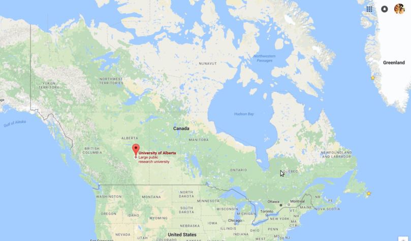
Figure1. Google map showing the locations of the University of Alberta, Canada.

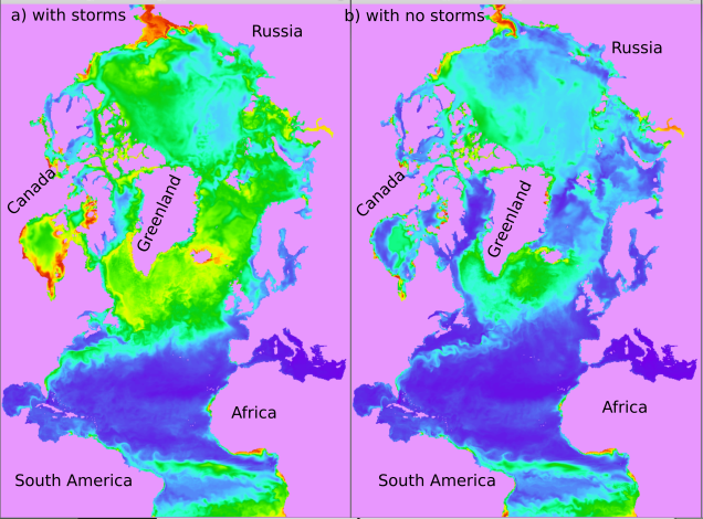
Figure 2. A simulation with storms (a) compared to a simulations without storms (b). The differences between each panel shows the regions where the storms have a greater impact on phytoplankton.

Calling all OSNAP collaborators and inspired oceanographic community members! OSNAP is looking for a new visual identity and is seeking your help in designing a creative logo.

How to Enter the Contest
The contest begins on October 1, 2016. Submissions will be accepted through November 15, 2016. Winners will be notified, and announced via our website and through social media. In order for your entry to be submitted and reviewed, please follow the details below:

1. Submit entry to Sarah Clem (sarah.clem@duke.edu)
2.  Submit the entry in its original source file and
3. Submit as a pdf with 300 dpi or higher.

Logo Requirements

• Design: The logo will be featured on our website, on our social media platforms and other media (e.g., research posters and t-shirts). Thus, we want the logo to be eye-catching, but also legible. Also, the logo should be easily reproducible and scalable for large and small formatting.
• Color: Any colors may be used. However, the logo should look good in color (if used) and in black and white.
• Integrity: Logos cannot contain copyrighted material. Logos must have been created by the contestant(s). Logos may not include images or licensed images that have been previously published.

Contestant Agreement
The winning contestant must agree that OSNAP can use their logo for future publications and outreach get ambien prescription applications. Additionally, the contestant must agree that OSNAP can alter, modify or revise the logo as it sees necessary. OSNAP reserves the right to not select a winner if, in its discretion, no suitable entries are received.

Prize
Contest winner will receive an Amazon Gift Card (and bragging rights!).

We want to bring everyone’s attention to the launch of the OSNAP Challenge located on this site under News and Events. Anyone is welcome to submit a prediction (or technically a hindcast because the data have already been collected) for the first two years of AMOC data from the OSNAP line. This contest is similar to the one organized by the RAPID program last year but in this contest there are no past observations of the AMOC from the OSNAP line so the level of difficulty is higher!

We are going to open up this blog to write-ups of the methods from each prediction and will be announcing the winners here in the Spring. The deadline for the submissions is April 1^st. For more information including instructions on how to submit a prediction and how the submissions will be judged, see the site here.

We wish everyone luck and may the best model win!

-Nick

OSNAP collaborators have a produced a order neurontin over the counter new paper for publication in the Bulletin of the American Meteorological Society. An early online release version of “Overturning in the Subpolar North Atlantic Program: a new international ocean observing system” is currently available on the AMS website:  http://journals.ametsoc.org/doi/abs/10.1175/BAMS-D-16-0057.1

by Ryan Peabody

Scientists and marine technicians have long appreciated the productivity-increasing role of caffeine [citation needed]. However, quantitative assessments of caffeine consumption and usage among the members of the DY054 science team have not yet been performed. Herein, we perform a not-quite-exhaustive nine-day analysis of tea and coffee consumption on the RRS Discovery. No significant trends were observed, other than a general preference for tea over coffee, and a sharp decrease in enthusiasm for the study as it progressed. Further work is needed to determine whether or not bush tea counts as a cup of tea, and exactly what quantity of coffee counts as a colloquial “cup.”

 Data were self-reported via “marker and whiteboard,” following methods developed in Mrs. Cooper’s second grade class [Cooper et al., 1999]. Logging was originally intended to take place daily at 23:59:59 UTC, but the lead scientist occasionally felt “really over it” and data were not recorded until the following morning. Efforts were taken to ensure that subjects maintained standard patterns of caffeine consumption, though it is worth noting that several believed the study to be a contest to see which one of them could drink the most coffee.

 Coffee and tea consumption demonstrate a general downward trend over the nine days, both passing a Mann-Kendall test (Figure 1). A 0.377 coefficient of cross-covariance implies that coffee and tea consumption are not related at any reasonable confidence level. Tea was consumed in generally higher quantities: on average 2.1 cups/person/day to coffee’s 1.6 cups/person/day. Further study is needed to determine if this is standard on a British flagged research vessel. Initial data supports this hypothesis: American-born members of the science team consumed 2.8 cups coffee/person/day and 1 cup tea/person/day, while British nationals consumed 1.3 cups coffee/person/day and 2.2 cups tea/person/day. The sole Hungarian-born member of the science team consumed an average of 6.1 cups of tea per day and 0 cups of coffee.

 Over time, a noticeable lack of enthusiasm for the study is evident, with participation dropping from 14 initial participants on day 1 to 6 participants on day 9 (Figure 2). On a ship with 45 crew and scientists on board, this represents a drop from “low” to “very low” participation. Despite the decrease, 70% of participants reported feeling “fair” to “good” about their own caffeine consumption and the study, indicating that maybe no one was really paying attention to the study in the first place. A least-squares fit of a nonlinear model of form b(1) + b(2)*exp(b(3)*t) represents the data very well, but also indicates that it was wise to end the study on day 9 (Figure 3). If the study had continued until the scheduled arrival in Southampton, approximately -15.5 responses would be logged each day, indicating that study participants would begin to erase the previously collected data, invalidating the entire study.

 Clearly, further study is needed to determine: 1) exactly how much caffeine is being consumed on board, 2) why no one wants to log their daily caffeine consumption, and 3) whether or not this was a good use of my time. Caffeine is a widely-consumed but little-studied product in the context of oceanographic research vessels, with most scientific effort going toward measurements of physical, chemical, and biological properties of the ocean. Though oceanographic research vessels are built and used primarily for the latter three areas of research, there is no apparent reason not to also study caffeine consumption.

Images by Ryan Peabody

by Femke de Jong

August 2, morning:

Today we, the NIOZ team, get to recover the first mooring. This particular mooring is not really part of OSNAP, it was originally deployed in 2003 as part of the Long-term Ocean Circulation Observations or LOCO project. It has been here ever since, except for a day or two between recovery and redeployment every summer.

LOCO is located on the 3km isobath on the western side of the Irminger Sea, right underneath a meteorological feature called the Greenland Tip Jet. This enhanced barrier wind that extends over the ocean causes very strong cooling in this region in winter. It’s what causes the warmish, salty surface water to cool, increase in density, and mix with the waters below. With LOCO we have a twelve year record of that mixing and we can study how it relates to the wind forcing and general changes in the Irminger Basin. As I’m writing this we’re steaming to LOCO to recover the thirteenth year. We’re hoping this will be our lucky number. Roald and Yvo have prepared everything on deck and in the last couple of days I’ve tested all my processing scripts. We’re all ready to go.

August 4, update:

We arrived at the LOCO position at 16:00 and started the mooring recovery. Because of the long stretch of empty cable (2400 m for the profiler) it’s quite a boring recovery. Mostly some instruments to get out at the beginning and end. All was on deck around 19:30. 

Roald and I have installed ourselves in the NIOZ container that was put on board before leg 1. We spend most of the rest of the day there reading out and re-programming the instruments. All of the instruments were still recording, so none of them ran out of batteries. That’s very comforting for us as this time they will go out for two years rather than one and it gives us some confidence that the estimates of how long they will run are correct. We stopped servicing at midnight to get some well-deserved rest.

Back to programming after breakfast. All the instruments had fresh batteries and programming around 10:30 so we started the mooring deployment. The anchor was dropped around 13:30. The final act consisted of a trilateration of the mooring position by ranging the distance to the anchor releases from several points around the mooring, which gives us the exact position of where we’ll find our friend in 2018. In the meantime we’ll let the instruments record some interesting things.

LOCO

Photos by Femke de Jong

by Mia Taylor

Since reaching our first CTD station near the coast of Greenland in the early hours of Saturday morning, things have switched up a gear and work is well underway.

One of the first CTD stations was in close proximity to the southern tip of Greenland, many of us were contemplating waking up in hope of seeing Greenland’s cliffs but the ETA for reaching it was 2am, meaning that it would be dark at this time and unlikely. However, during the night the schedule shifted slightly and we reached the station closest to the coast around 5am, just as dawn was breaking. Despite lots of cloud and a grey hazy sky, the coastline was visible. We could see the flashing light from a lighthouse at Prince Christian Sound and to its left there appeared to be a glacier, further left again, a large iceberg. The glacier was intriguing, it was the brightest thing on the coastline yet with the poor visibility it was hard to understand visually; was it receding into the mountain or a layer of ice cloaking or jutting out of the cliff? No amount of squinting could clarify this for me. Most curious was that it was sparkling, as if it was covered with a gentle sprinkling of glitter.

Yesterday – Sunday – the moorings began; M1 and M2 were recovered, having been underwater and actively collecting data for the past year. This is the first time OSNAP have returned to the moorings since they were deployed so bringing them to the surface and retrieving their data was an exciting prospect, as was seeing their condition for the first time since spending a year beneath sea level. Recovering the moorings requires hauling them out of the ocean and removing and cataloguing the instruments. It’s heavy work and it’s cold out, plus due to the high pressure in the area the waves are rolling with more swell than the last couple of days, but the NMFS technicians who are organising the operation have the process efficiently choreographed and everything ran smoothly. Once all of the M1 and M2 2015-16 moorings were out of the water (all of which were fine, with the addition of some biology to a few buoys) a reconditioned set were ready to go back in. If you are not familiar with what these mooring’s are, let me try and explain: one mooring includes groupings of about four buoys incrementally attached along a long line of wire and between these groupings data collecting instruments are further attached.
Many of these instruments look cylindrical and are made from a combination of metals to prevent corrosion. The wire is long – M1 was 2059m in length – at the end of the wire a heavy weight is attached, which is designed to sink to the seabed pulling the wire and the buoys down with it so the line and buoys float vertically upwards, securing the instruments for data collection at
different depths. When it’s time for the mooring to return to the surface for data collection an acoustic release mechanism triggers the wire to detach from the weight and due to its buoyancy the mooring floats back up to the surface. M1, M2 and now M3 reached the surface intact and untangled making it easier for a technician to catch it and draw it back to the ship.

To successfully drag down the buoys the weight needs to be significant, for the redeployed M1 and M2 moorings a small part of a massive anchor chain had been chosen, to give an idea of its scale, each chain link is about the width of my forearm. It made a dramatic sight when held aloft by the winch and hanging between the gantries before it was dropped to its watery grave.

In the evening, having completed work at moorings M1 and M2 the ship headed back closer to Greenland for more CTD stations and the launching of a number of RAFOS floats. Sotiria and Ryan – who are on the 12am – 12pm watch – and the technicians spent the early hours consistently busy preparing the CTD, collecting water samples for salinity and nutrient analyses and recording details for the watch log. Although it is the middle of the night, it’s a nice time to be up and about. It’s more peaceful and the pitch black of the night sky against the bright lights of the ship sets an atmospheric scene. Even though it’s not possible to see the vast expanse of water around us at that time, you can definitely feel it. As dawn breaks (around 5am), wandering up the outside stairwells it seems there is always someone to run into who is starting their day.

Punctuating the work and giving structure to the day are mealtimes; the food is fantastic and includes more options than could possibly be eaten at one sitting. Should it be possible to lose sight of what day it is (I think it is possible), the meals offer each day a sense of identity; fish on Friday and today, Sunday, we had a roast dinner (with amazing spuds). The galley is indicative of how things seem to run on the Discovery as a whole; the standards are high and everyone is friendly. As a first-timer on a ship it’s crystal clear that everyone works very hard and that things run like a well-oiled machine. Everyone is doing different shifts so there is always someone awake and alert; it’s a 24hour ship in every respect. Options for downtime apart from socialising or having the sea rock you to sleep, include a session at the gym, playing cards or Wii, watching a video, or a number of other things, including perusing from library’s collection. One of its gems is ‘A century of Discovery’, charting some of the Discovery’s past voyages from the last few hundred years. Interesting fact: Captain Cooks ship, The HM Sloop Discovery, weighed 229 tons*, compare that to the 2012 RRS Discovery, which weighs around 6000 tons. The sense of history attached to the Discovery is inescapable here as photographs and prints of ships bearing the ‘Discovery’ name are hung on the walls of each deck, and show majestic looking ships alongside explorers, ice and penguins. It is a profound reminder of the ships heritage and that the vessel and its people are integral cogs in continuing its legacy of exploration and pioneering research, enabling new knowledge to inform our lives.

Other excitement on board today included Ian, the purser, opening the bond (theship’s shop) where you can buy chocolate, sweets, cigarettes, clothing bearing the ‘Discovery’ logo and more, within minutes of opening there is queue. More exciting again (if possible), this morning we saw a group of pilot whales to the side of the ship. They didn’t hang around but hopefully they will be back.

* Ships employed in Arctic ice: Discoverys past, 1602 to 1876 by Ann Savours, Archives of Natural History, 2005, A century of Discovery, Volume 32 Part 2

Peter, Wallly, and Tommy

Discovery in the Arctic

Mooring weight chain

Night CTD

Greenland coast

Mooring instrument

Photos by Mia Taylor

by Penny Holliday

RRS Discovery cruise today left Reykjavik on what surely must be the most beautiful day of the year so far. Sailing into glaring sunshine over blue sparkly water brings a optimistic lift to the heart of this Principal Scientist – it almost makes you think that we won’t need all of those extra days we have scheduled in case of delays due to bad weather… But the bad weather will probably come at some point, so I wont yet get too carried away with talking about calm conditions.

Most of us have spent a few days in Reykjavik, getting excited by seeing four research vessels in port at the same time (surely quite unusual?), gasping at the price of shopping, and admiring this stylish city in all it’s crazy-weather glory. But now we are glad to be getting going and getting on with the task ahead of us.

This cruise DY054 is the second UK OSNAP mooring refurbishment cruise of 2016. We’ll be retrieving some moorings and instruments that have been collecting deep ocean data for the past year, and sending a new lot of instruments back to replace them. We’ll also be releasing some ocean-exploring robots – floats that will spend two years following the coldest and deepest water so we can trace the many ribbons of currents that make up the southward-flowing circulation.

Reykjvik

Reykjavik

R.V. Neil Armstrong

RRS Discovery and RV Maria S Merian

RV Bjarni Saemundsson

Reykjavik

Photos by Penny Holliday

by Feili Li

It has been two days since we left Reykjavik and we are heading southwestward to the Irminger Sea, east of Greenland.   It will take about another day before we reach the location of the first CTD station near the Greenland side.   So before we get there, let me explain several things: who we are, why we are in the cold subpolar area, and what we are doing before getting to the working site.

We are a group of enthusiastic hard-working researchers coming from seven institutions and four countries on a research cruise aboard RRS Discovery.  Here the word “researcher” is preferable to “scientist” because we have an artist Mia and a photographer Amanda onboard – we are all doing research, just in diverse disciplines.  (If you are as interested in their work on the cruise as I am, stay tuned to our blog!)  Below are some nice photos of us.

One of the main goals of this research cruise is to retrieve data (sea water temperature, salinity, and current velocity) from the moored array as part of OSNAP, which has been sitting in the Irminger basin for another full year.  After the data retrieval, moorings will be redeployed and will be staying in the water for the next two years.  Processing of the data will begin shortly after they have been collected, although it may take several months to finish the processing and quality control of all these data.  With the data, we are one step further towards the first result about the overturning circulation in the subpolar North Atlantic.  It will provide unprecedented opportunities for understanding how water masses formed at high latitudes are tied to large scale Atlantic circulation that relates to climate change and variability.

Before getting to the site, we are generally free.  I feel like I have moved my office from Durham in North Carolina to the ship.  Except for training on CTD watch, I have been basically working on my laptop in a lab with a nice ocean view.  The boundary between work and life disappears:  eat, tea, work, eat, tea, work, eat, eat, eat … Yes, the boundary between the times you are eating and the times you are not eating also disappears.  But, soon, this will be substituted with days filled with lifting, walking, taking water samples, and that is when the real game starts.

Photos credit:  Neill Mackay

press release

A new record in mixing of surface and deep ocean water in the Irminger Sea has important consequences for the Atlantic overturning circulation 

Scientists Femke de Jong and Laura de Steur of the NIOZ Royal Netherlands Institute for Sea Research have shown that the recent temperature changes in the Irminger Sea between Iceland and Greenland can be explained through regional ocean-atmosphere interaction during the cold winter of 2014-2015. This rejects a hypothesis that posed that increased meltwater from Greenland weakened deep water formation and caused the cold blob. The article by de Jong and de Steur is accepted by Geophysical Research letters and has appeared online.

Continue reading →