Author Archives: Sarah

First Float Results from OSNAP

By Amy Bower and Heather Furey

During the summer of 2014, the first setting of 40 deep acoustically-tracked RAFOS floats was made along the OSNAP line (see Mysteries of the Deep Subpolar North Atlantic). Most of these floats were programmed in advance to stay submerged for two years, all the time drifting passively with the deep currents. However, a few floats were programmed for only 180 days so that we could determine how the sound sources are working and how well we were able to adjust the floats’ weight so that they drift just about 100-200 m above the sea floor. Believe it or not, a half year has already passed since the floats were deployed, and the three scheduled to surface after that time have done so over the past few months.

The data collected by these floats indicate that the sound sources all seem to be working properly. The floats were not able to hear the sound sources continuously because of the extremely rough topography of the Reykjanes Ridge, the submarine mountain range that extends southwestward from Iceland forming part of the mid-Atlantic ridge system. Sometimes the floats drift behind underwater mountains that prevent the acoustic signals emitted by the sound sources from reaching the float. This can lead to a short gap in our knowledge of where the float was during that time. This is completely expected and we can usually interpolate the float position during the time it is “invisible”.

Continue reading

Unravelling the sensitivity of Atlantic overturning to past forcing

by David Marshall

Fundamental questions we would like to answer in OSNAP are how changes in wind, thermal and freshwater forcing over the subpolar Atlantic modify the Atlantic Meridional Overturning Circulation (AMOC) at lower latitudes and on what time scales? These teleconnections are hard to unravel due to the complexities of the three-dimensional ocean circulation.

A conventional approach to addressing such questions to take a state-of-the-art ocean circulation model and modify the surface forcing in a large number different locations at different times in the past. The problem with this approach is that there are literally thousands of wind, thermal and freshwater forcing anomalies that we need to consider, each requiring a separate model integration.

An alternative approach, which we have used to interpret the AMOC time series at 26.5oN from the RAPID-MOCHA array, is to use an adjoint model (Pillar et al., 2015). The basic idea of an adjoint model is both simple and surprisingly subtle. Rather than run the model forwards in time, we run it backwards. In a conventional forward model, you perturb the initial conditions, for example, the wind forcing at some time in the past, and see how the three-dimensional circulation evolves differently at all times in the future. In an adjoint model, we purturb a single output, for example the AMOC at 26.5oN, and by run the model backwards to see how that output is sensitive to all forcing anomalies in the past.

Continue reading

Visualising changes in the North Atlantic ocean

by Ric Williams – University of Liverpool

Animations of the observed changes in the physical properties of the North Atlantic can really help us to understand their geographical distribution and their evolution over time. We’ve created a series of animations of different properties, and here show a few to give you a flavour of the insight they provide. You can see more on our YouTube Channel.

The North Atlantic Ocean anomaly animations are based on a reanalysis of historical temperature and salinity data by Dr Doug Smith at the UK Met Office, where the sparse observations are mapped using model covariances from a Hadley Centre model (Smith and Murphy, 2007). The plots are made by Dr Vassil Roussenov and the videos by Dr Andy Heath, and Prof. Ric Williams (all from the University of Liverpool) is the lead investigator; this work was supported by the UK Natural Environment Research Council.

This is an animation of annual anomalies of ocean heat content (10^8Jm^-2) over the North Atlantic, where red is warm and blue is cool. The annual anomalies are defined relative to a time average from 1950 to 2010, and are evaluated for the full ocean depth. The animations reveal the strong interannual and decadal variability. There are often different responses occurring in the subtropical and subpolar gyres (Williams et al., 2014), as well as occasions when thermal anomalies appear to pass from one gyre to the other. At the same time, there is an overall warming trend over this 60 year period, represented by the anomalies becoming warmer over the last decade. The different decadal responses are emphasized by the pictures of the time-averaged thermal anomalies for 1950-1970, 1980-2000 and 2000-2010.

The mechanisms forming these ocean heat content anomalies involve the imprint of changes in wind forcing, physical transport and redistribution of heat within the basin, and local and far field changes in air-sea heat fluxes. The dominant mechanisms probably vary with the location and timescale of interest.

Sea surface height varies for a range of reasons. Atmospheric forcing induces waves and even storm surges, while gravitational effects of the Moon and Sun induce the predictable tidal undulations in sea level. The sea level also responds to the heating and cooling of the ocean, sea level increasing from the water column expanding when the water warms or freshens. The sea level likewise increases from the addition of mass from more water added to the global ocean from river runoff and melting of ice on land.

The animation shows the annual sea surface height anomalies in sea level (mm) in the North Atlantic calculated from how the water column expands when there is warmer or fresher water. The sea level varies by -50 mm (blue) to +50 mm (red) due to these volume changes. The animation reveals a similar response to ocean heat content change, regions of heat gain associated with a higher sea level (red) versus regions of heat loss associated with a lower sea level (blue). Again there is strong decadal variability for the ocean gyres, as well as a background rise in sea level over the entire record.

The mechanisms forming these sea surface height anomalies involves the imprint of changes in wind forcing, physical transport and redistribution of heat and freshwater within the basin, and local and far field changes in air-sea heat and freshwater fluxes. The dominant mechanisms probably vary with the location and timescale of interest, although much of the local variability is likely to involve a redistribution of warmer and lighter waters.

Sea surface temperature varies due to solar heating and air-sea exchange of heat, as well as due to transport of warm waters and mixing with cooler, deeper waters.  The animation shows the annual anomalies in sea surface temperature (C) in the North Atlantic, varying from -1.5C (blue) to +1.5C (red). The animation is broadly similar to the ocean heat content change, regions of higher sea surface temperature generally coinciding with greater ocean heat content, although there are detailed differences, particularly in the subtropical latitudes. Again there is strong decadal variability for the ocean gyres, as well as a recent surface warming for 2000 to 2010.

The sea surface temperature (SST) anomalies are generally viewed as being driven by anomalies in air-sea fluxes on interannual timescales (greater heat input from the atmosphere leads to warmer SST), but might feedback back and determine the air-sea fluxes on decadal or longer timescales (a warmer SST leads to a greater loss of heat from the ocean to the atmosphere). There is also a physical transport of the SST anomalies on all timescales.

What are the seagoing scientists doing now?

Penny Holliday, NOC

Many of the OSNAP blog stories we’ve posted so far give a flavour of the exciting array we have deployed in the subpolar North Atlantic, and the process by which we have achieved this. With a fleet of 4 ships and a diverse teamP1010183 of scientists and engineers, over the course of the 2014 summer we put in place our measuring system that will tell us so much about the circulation of the region. Many of our instruments lie unattended and uncommunicative in the darkness of the deep ocean until we haul them out of the depths and back into fresh air one or two years later. We harvest the data as soon as they come back onboard and the long process of turning a large set of numbers into information about the changing ocean begins.

So you might think that now the instruments are in the water we can take a break, do something else, and just wait for the next cruises to come along. Or you might guess the truth, which something rather different. The detailed planning for next years’ cruises has already started, and work on data collected during the array deployment cruises, and from instruments that are communicative while they roam the ocean, is well underway.

Continue reading

What is the real puppet master of the AMOC variability?

By Xiao-pei Lin

“AMOC, consisting of a northward flow of warm surface waters and a southward flow of cold deep waters, is the leading mechanism for heat transport and carbon sequestration in the Atlantic Ocean,” said Macdonald and Wunsch in 1996.

As the key component of global meridional overturning circulation, Atlantic Meridional Overturning Circulation (AMOC) plays a significant role in modulating the global climate system, which has drawn continuous attention from oceanographers for decades. However, increasing knowledge on the AMOC has not clarified its nature, but led us to more confusion.

Studies on the mechanism of AMOC can date back to 1950s, when AMOC was viewed as a source/sink-driven overturning cell and often simplified as a conveyor belt for exporting the deep water formed in the high latitude of the North Atlantic to the low latitude and South Atlantic. Variability of the AMOC was supposed to be controlled by either the source, i.e., the production of deep water, or the sink, i.e., the return of deep ocean water to the surface. This simple framework has been dominating our society for decades.

However, this traditional view has been challenged lately by a number of studies. Dr. Jian Zhao, who just completed his doctorate from University of Miami, suggested seasonal cycle of AMOC, and a large part of AMOC interannual variability at 26.5°N, are controlled mainly by wind forcing. Jiayan Yang, a PI from Woods Hole Oceanographic Institution, says,“Recent work shines light on that it is the wind stress not the buoyancy flux that is the leading mechanism for AMOC variability from seasonal to interannual, even decadal time scales.”

Continue reading

Welcome OSNAP Students and Postdocs

by Susan Lozier

As the swift pace of the OSNAP field season has wound down, we have been gathering profiles of the students and postdocs who are working on OSNAP projects.  So, with this post I would like to welcome those young oceanographers: Till Baumann (GEOMAR, Helmholtz Centre for Ocean Research), Elizabeth Comer (National Oceanography Centre and University of Southampton), and Nick Foukal and Sijia Zou (Duke University) are graduate students working on OSNAP projects and Loïc Houpert (Scottish Association for Marine Sciences) and Neill Mackay (National Oceanography Centre) are postdocs.  See:  http://www.o-snap.org/partners/students-postdocs/ for more information about these oceanographers and their projects.  As with almost all other large scale ocean observational programs, OSNAP was designed by those of us who have been oceanographers for a number of years, if for no other reason than the planning itself can take a number of years. Continue reading

Ocean University of China’s first observation experience in the North Atlantic

by Xiaopei Lin and Dexing Wu

“Pay out the wire slowly and keep it tense in the water, okay?”

“Got it!”

“Okay, go ahead.”

It was another foggy and calm morning in the Subpolar Atlantic onboard the R/V Knorr. John Kemp, the mooring group leader, was teaching Chun Zhou, a physical oceanography PhD student from China, how to drive the winch to lay the mooring wire rope into the water. Almost two months have passed since the end of that cruise. However, some people may still remember Dalei Song, Xiaoman Yang, and Chun Zhou, the three Chinese guys on board who were there representing the Ocean University of China (OUC) and making the university’s first move in cooperation with partners as one of the members of OSNAP.

OSNAP is a US-led international collaborative project designed to provide a continuous record of the full-water column, trans-basin fluxes of heat, mass and freshwater in the subpolar North Atlantic using a network composed of moorings, ship-based hydrographic sections, RAFOS floats and gliders. As planned by the principal investigators, the objective for Cruise #Kn221-03 was to deploy moorings, carry out several high-resolution CTD sections, and deploy dozens of RAFOS floats. Taking into consideration the OUC participants’ experience with mooring operation, Dr. Bob Pickart, the chief scientist of this cruise, assigned them to John, who led a small group comprised of the best hands in mooring operation. Continue reading

To Sea with Less

by Susan Lozier

Late last month I attended a symposium in London celebrating the tenth anniversary of the UK-US RAPID array at 26°N in the subtropical North Atlantic. All assembled agreed that this first continuous measure of the ocean’s meridional overturning circulation has produced a dramatic shift in our understanding of the large scale ocean circulation in the North Atlantic. Those of us working on the OSNAP project understand all too well that with this dramatic shift RAPID has set a high bar for success. So, to all RAPID PIs, let me offer a congratulatory note on behalf of all OSNAP PIs on this milestone. Well done.

For those of us involved in these large scale ocean observing programs, we have little to no doubt as to their benefit to our science in the sparklingshort run, and to society in the longer run. But these observations come at a price that is sizable to most any funding agency. This price tag, coupled with the dawning realization that we will need to measure for years and years in order to discern long term trends of the overturning and its attendant heat, carbon and freshwater fluxes, should give us pause. This message more or less was delivered to those assembled in London in the closing remarks given by Professor Duncan Wingham, Chief Executive of the UK National Environmental Research Council (NERC). Professor Wingham noted the irony of an Environmental Research Council funding ships to crisscross the ocean all the while burning (lots of) fossil fuels. It is though the cost of business and oceanographers can hardly be held responsible for the rising cost of fuel over this past decade. And yet, all of us understand that with anything the price must be commensurate with the value added. While we as oceanographers are convinced of the value, I think it is safe to say that outside of our community it may not be so patently obvious. Continue reading

Northern gliders linking OSNAP and Vitals

Northern gliders linking OSNAP and Vitals

Brad deYoung, Jaime Palter, Ralf Bachmayer, Robin Matthews, Tara Howatt, Brian Claus – Memorial and McGill Universities

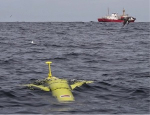
CSS Hudson in the background as the glider is inspected by  seabirds.

CSS Hudson in the background as the glider is inspected by seabirds.

At Memorial we are active not only in OSNAP, but also in Vitals a different program with a focus on air-sea gas exchange in the Labrador Sea. So a sibling program to OSNAP. This year is still preparation for the main field season next year in 2015. We wanted to deploy the three gliders this year to explore the along-shelf variability of the cross-shelf character of the Labrador Current at the shelf-break, to learn more about flying multiple gliders at once, to gain more experience with the 1000m glider and learn more about new gas sensors. We were also very excited to link our two programs by flying the gliders along the shelf-break through the 53 o N mooring array.

Our gliders went out in early July. Our plan was to deploy the three gliders and have two criss-crosses the shelf break, surveying the shelf-break Labrador Current, while the third glider sampled inshore on the inner side of the current. This did work, but not quite as well as we had planned.

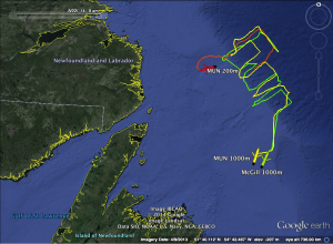
Picture  2

Three gliders were deployed, one shallow (200m – red) and two deep (1000m – yellow and green).

The deployment was from CSS Hudson for which we thank our colleagues Blair Greenan and Dave Hebert at the Bedford Institute of Oceanography. This was the same cruise on which the Canadian OSNAP moorings were deployed. The zigzag plan did mostly work but we had to recover one glider early because of a leak problem and the others had some troubles with lighter than expected water at the surface on the shelf. The gliders were in the water for about six weeks, about four weeks short of our intended deployment.

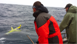
Beyond some cool data, that we are now looking at, we learned some things about flying multiple gliders in strong currents, we improved our IPad App that allows us to monitor the gliders, and we learned some new things about gliders behaviour. As it turns out, if the glider is coming to the surface but is a little too heavy and so only makes it to 7 m depth (that is not really very good, no surfacing no communication no GPS fix) then the glider is happy and does not conclude that there is a big problem. So it does not get upset and drop its emergency weight to force its way to the surface. Our two heavy-weight gliders did eventually conclude there was a problem, but for another reason, and dropped their weights. We then had to arrange a ship to head out to the shelf break to pick up the gliders turned into surface drifters. The good news is that glider recovery does not require a hugely complicated set of instruments (see picture) and fishing boats are pretty much perfect for the task and fishermen are very good at finding and retrieving things on the ocean.

Key tools for a glider recovery.

Key tools for a glider recovery.

As it turned out, the weather cooperated and we had good positions, and so the recovery went very smoothly. We did also try to recover another lost instrument, an Ocean Bottom Seismometer, deployed by our German colleagues and adrift with two years of data inside but we were unable to find it as the Argos positions were too stale or inaccurate and we just could not find it. That was very frustrating. We knew where it was but not well enough to find it. The good news for our gliders is that in finding them they still had lots of battery power left and so after a little refurbishment they were ready for another deployment. You can’t hold a good glider down, or up – what is that expression? More on the second deployment in our next blog entry.

Finding a lost glider and bringing it home.

Finding a lost glider and bringing it home.


“Dinnae expect onything an ye’ll no be disappointed”

Four Decades of Weather and Climate at the Scottish Association for Marine Science Laboratory on the Dunstaffnage Peninsula in the Scottish West Highlands (1972 to 2014)[1]

Stuart Cunningham, 29th July 2014

“Of mice and men” stated that the arguments about the causes of climate change are settled (in the same way we no longer argue whether the Earth orbits the sun): climate is changing and it is our doing. Practically we need to focus more on the regional impacts of climate change. The OSNAP programme will provide such a focus. This article describes some regional climate – in the west highlands of Scotland, linking this to global climate teleconnections and climate change. We then describe briefly how OSNAP contributes to new knowledge and understanding of how regional climate and wider climate patterns can be linked.

Within the grounds of the SAMS marine laboratory, at Dunstaffnage, the UK Meteorological Office maintains a synoptic weather and climate station. Operating continuously since 1972 we can now investigate climate at this site over four decades. What does it show about the weather and climate in the west highlands of Scotland?

The seasonal cycles of air minimum and maximum temperatures, rainfall, sunshine hours and air-frost days (Figure 1, Table 1) have clearly defined seasonal variations. Our summers are warmest in July and August, but sunniest in May, and notably dry in April, May and June. Overall, we have a wet climate, with an annual average rainfall of 165 cm (5 feet 5 inches for the imperialists amongst you!). But the variability of our weather (and the beauty of our geography) gives a special meaning to fine days. Alastair Reid’s poem “Scotland” perfectly captures the mood swings of the Scottish psyche induced by the Scottish climate (and the Calvanism). For your edification the poem is reproduced at the end of this blog.
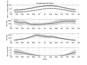
Figure 1: Seasonal cycle of monthly mean temperatures (°C, minimum dashed, maximum solid), rainfall (mm), sunshine hours (hrs), days of air-frost (days). The monthly mean temperature is calculated from the average of the mean daily maximum and mean daily minimum temperature i.e. (tmax+tmin)/2.Shaded region is one standard deviation of the monthly mean. The seasonal cycle has been computed from January 1972 to Feb 2014 except for sunshine hours, recorded in two periods: from September 1981 to September 1984 (three years) and from March 1986 to December 2001 (16 years). All the meteorological data analysed here can be downloaded freely from www.metoffice.gov.uk/public/weather/climate-historic/#?tab=climateHistoric.
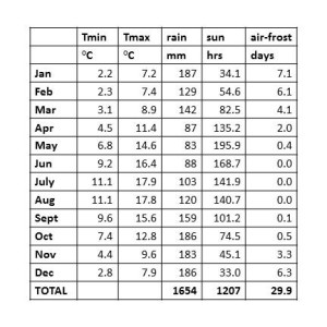
Figure 1: Seasonal cycle of monthly mean temperatures (°C, minimum dashed, maximum solid), rainfall (mm), sunshine hours (hrs), days of air-frost (days). The monthly mean temperature is calculated from the average of the mean daily maximum and mean daily minimum temperature i.e. (tmax+tmin)/2.Shaded region is one standard deviation of the monthly mean. The seasonal cycle has been computed from January 1972 to Feb 2014 except for sunshine hours, recorded in two periods: from September 1981 to September 1984 (three years) and from March 1986 to December 2001 (16 years). All the meteorological data analysed here can be downloaded freely from www.metoffice.gov.uk/public/weather/climate-historic/#?tab=climateHistoric.

Table 1: The Seasonal Cycle values of monthly mean values of minimum and maximum temperature, (°C) rainfall (mm), sunshine (hours) and number of air-frost days (days).

Table 1: The Seasonal Cycle values of monthly mean values of minimum and maximum temperature, (°C) rainfall (mm), sunshine (hours) and number of air-frost days (days).

Climate Trends

We will look now at long-term weather trends of temperatures and rainfall (i.e. the climate). These two variables have quite different patterns of change over four decades, nicely illustrating the complexity of climate.

Temperature

The singular striking aspect of the temperature anomalies at Dunstaffnage (Figure 2) is the pattern of cold anomalies between 1972 and 1995, which are completely reversed to warm anomalies between 1995 and 2010. A linear trend shows a warming of 1.08°C from 1972 to 2014. Shown in the plot are the 95% confidence limits for this trend.
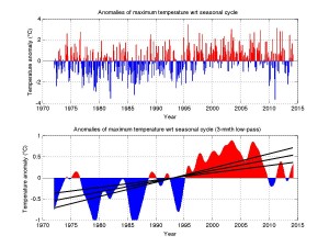
Figure 2: Anomalies of maximum monthly mean air temperature (°C) relative to the seasonal cycle. Top panel shows monthly values and the lower panel 3-month low-pass filtered values. In the lower panel the solid line is the linear trend of the anomalies with 95% confidence intervals. Anomalies of minimum monthly mean air temperature (not shown) are almost identical in monthly pattern and long-term trend. The trend is 1.08°C calculated between 1972 and 2014. This is a trend of 0.26°C/decade.

Figure 2: Anomalies of maximum monthly mean air temperature (°C) relative to the seasonal cycle. Top panel shows monthly values and the lower panel 3-month low-pass filtered values. In the lower panel the solid line is the linear trend of the anomalies with 95% confidence intervals. Anomalies of minimum monthly mean air temperature (not shown) are almost identical in monthly pattern and long-term trend. The trend is 1.08°C calculated between 1972 and 2014. This is a trend of 0.26°C/decade.

How does this local temperature change compare to global average temperature changes? Over Earth’s land and ocean surface the average temperature is increasing rapidly: the warming (by linear trend) from 1972 to 2014 is 0.8°C[1]. Most of the observed increase in globally averaged temperature since the mid-twentieth century, is very likely due to a 40% increase in atmospheric carbon dioxide concentration since the pre-industrial era[2]. Dunstaffnage temperatures have risen by 1.08°C, therefore increasing at a rate 26% higher than the global average. Quite possibly this more rapid warming at Dunstaffnage (56.4545° N, 5.4379° W) is linked to the amplification of warming at high latitudes due to decreasing ocean ice cover (amongst a host of other potential feedbacks). Changes in northward heat transport by the oceans and moist atmosphere could also be implicated.

In the last decade global average temperatures have remained constant or decreased slightly, and this is reflected in decreasing temperatures after 2007 at Dunstaffnage (Figure 2). This temperature stand does not mean an end to global warming, but is explained by natural climate variations: large cyclic variations in North Pacific winds[3] have increased heat absorption by the ocean, leading to steady atmospheric temperatures. We have not demonstrated a link between temperatures in Dunstaffnage and atmospheric variability in the Pacific, but it is probable.

Therefore at Dunstaffnage the long-term temperature trend strongly links to the global warming trend and to effects of preferentially increased warming rates at high latitudes. We also see evidence for remote effects of natural cycles of Pacific climate variability in the stand of warm temperature anomalies in the past decade.


 Rainfall

One difficulty with analyzing rainfall data is the large inherent variable. This is readily seen in Figure 2, as the large variation around the mean value in each monthly mean value of rainfall (the grey bars are large): it can be wet or dry at any time of the year with large variations around the seasonal (expected) value.
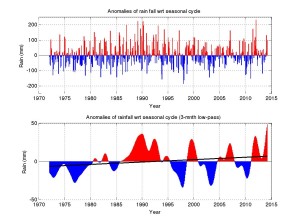
Figure 3: Anomalies of monthly mean rainfall (mm) relative to the seasonal cycle. Top panel shows monthly values and the lower panel 3-month low-pass filtered values. In the lower panel the solid line is the linear trend of the anomalies.

Figure 3: Anomalies of monthly mean rainfall (mm) relative to the seasonal cycle. Top panel shows monthly values and the lower panel 3-month low-pass filtered values. In the lower panel the solid line is the linear trend of the anomalies.

At Dunstaffnage (Figure 3) there is an approximately five-year cycle of wetter and drier periods (particularly since the mid-1990s). The long-term trend from 1972 to 2014 suggests a net increase in annual rainfall of 13 mm (3.1 mm/decade), but statistically this trend is not significant. Our inability to identify long-term trends of observed rainfall is a typical problem for the majority of global rainfall observations.

As an aside, a warming atmosphere holds more water vapor, the content increasing approximately 7% for one degree of warming. The oceans dominate the fresh-water cycle, evaporating 13 million cubic meters of water per second and receiving 12 million cubic meters of water per second in rainfall. The small difference of 1 million cubic meters per second falls as rain over the land. Changes in pattern and amounts of rainfall over the ocean change the oceans’ salinity and thus observations of ocean salinity can tell us about changing precipitation (the ocean rain gauge) – even if trends in rainfall are hard to detect by direct observation over the land.

Although rainfall at Dunstaffnage is an inherently noisy process we can relate it to the main pattern of atmospheric variability in the North Atlantic called the North Atlantic Oscillation (NAO). The atmosphere in the Atlantic has a high pressure centered over the Azores and a low pressure centered over Iceland. The atmospheric pressure difference from the Azores to Iceland strongly controls the direction and strength of weather patterns – the westerly trade winds – that travel from west to east across the Atlantic. When the pressure difference between the Azores and Iceland is larger than normal then storms tend to pass eastward at higher latitudes than normal (north of the UK in extreme cases). This leads typically to wetter (and warmer) conditions over west Scotland. Conversely, for a lower than normal pressure difference, storms track eastward at much lower latitudes, bringing rain to Spain: and dry (and colder) conditions to the west of Scotland.

Comparing rainfall at Dunstaffnage to the North Atlantic Oscillation Index (Figure 4), there is evidently some relationship: often the red (high NAO index/high rainfall) and blue (low NAO index/low rainfall) correspond. While the correspondence is not one-to-one, the variations in the NAO index explain 44% to 57% of the signal in Dunstaffnage rainfall (range is 95% confidence interval). Thus Dunstaffnage experiences rainfall patterns that are strongly related to the latitude at which the west to east moving storms cross the Atlantic.

Figure 4: (top panel) North Atlantic Oscillation Index. Normalized pressure difference between the Azores high pressure and Icelandic low pressure. Index downloaded on 12th March 2014 from the US National Centre for Environmental Prediction [www.cpc.ncep.noaa.gov/products/precip/CWlink/ENSO/verf/new.nao.shtml]. (bottom panel) Anomalies of rainfall (mm) relative to the seasonal cycle, at Dunstaffnage.

Figure 4: (top panel) North Atlantic Oscillation Index. Normalized pressure difference between the Azores high pressure and Icelandic low pressure. Index downloaded on 12th March 2014 from the US National Centre for Environmental Prediction [www.cpc.ncep.noaa.gov/products/precip/CWlink/ENSO/verf/new.nao.shtml]. (bottom panel) Anomalies of rainfall (mm) relative to the seasonal cycle, at Dunstaffnage.

We can extend our comparison of Dunstaffnage rainfall and the atmospheric variability over the Atlantic by thinking how the North Atlantic Oscillation and rainfall changes accumulate over time. That is do drier or wetter patterns persist for many years? To examine this we simply add the rainfall anomalies with time and do the same for the North Atlantic Oscillation Index (Figure 5).

From 1972 to 1986 Dunstaffnage became progressively drier with time (Figure 5). This makes sense looking at Figure 4 where these years have negative rainfall anomalies. Then we enter a wetter period from 1986 to a peak in rainfall accumulation in 1995. Since then Dunstaffnage is trending towards drier conditions, but with the 5-year oscillation evident. The accumulated oscillation index (Figure 5) corresponds closely with the rainfall accumulation. The oscillation index explains 67% to 75% of the signal in accumulated rainfall (at 95% confidence limits). This correspondence between the rainfall and the oscillation index is entirely expected. Hundreds of scientific papers have established links between the oscillation and multiple climate variables: analysis includes both modern data and paleo-climate data, establishing that this pattern has been active for at least 5000 years.
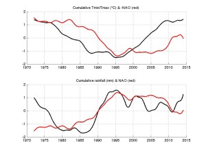
 

Figure 5: Cumulative addition of Dunstaffnage rainfall (black) and the North Atlantic Oscillation Index all months (red). Both timeseries have been normalized. Accumulating rainfall corresponds to increasing oscillation index.

Figure 5: Cumulative addition of Dunstaffnage rainfall (black) and the North Atlantic Oscillation Index all months (red). Both timeseries have been normalized. Accumulating rainfall corresponds to increasing oscillation index.

Discussion

At Dunstaffnage we can link local temperature and rainfall variability to patterns of established climate variability: rainfall to the North Atlantic Oscillation; temperatures to the Pacific Decadal Oscillation. We can also identify the global warming temperature trend at Dunstaffnage and find that it is larger than the global average temperature rise: we suggest this is related to more rapid warming that happens at higher latitudes.

Regrettably, I have falsified the title of this article “‘Dinnae expect onything an ye’ll no be disappointed”, by demonstrating that by examining data around the globe can tell us with some confidence what to expect, both for long-term temperature trends and for rainfall trends.

So can we better understand these global to regional teleconnections in weather and climate patterns? The Overturning in the subpolar North Atlantic Programme is measuring the circulation in the subpolar North Atlantic because there is mounting evidence that knowing the circulation in this region leads to improved decadal climate prediction. Both modelling and observations studies link temperatures and currents in the subpolar gyre to tropical storm and hurricane frequency, rainfall in the Sahel, Amazon, western Europe and parts of the US, on wind strength and on marine ecosystems.

Thus the contribution of OSNAP to this much wider climate forecast problem is to generate new knowledge and understanding of the subpolar gyre by measuring the circulation and fluxes of heat and fresh water from Newfoundland to Greenland to Scotland. This continent-to-continent observing system will enable the relationships between circulation, ocean and atmosphere exchanges and climate impacts, for the first time, to be examined with a purposefully designed observing system.

Progress is oftentimes by small steps, but occasionally extraordinary efforts to take leap forward need to be taken.

Scotland
It was a day peculiar to this piece of the planet,
when larks rose on long thin strings of singing
and the air shifted with the shimmer of actual angels.
Greenness entered the body. The grasses
shivered with presences, and sunlight
stayed like a halo on hair and heather and hills.
Walking into town, I saw, in a radiant raincoat,
the woman from the fish-shop. ‘What a day it is!’
cried I, like a sunstruck madman.
And what did she have to say for it?
Her brow grew bleak, her ancestors raged in their graves
as she spoke with their ancient misery:
‘We’ll pay for it, we’ll pay for it, we’ll pay for it.’
Alastair Reid

View as PDF

[1] This article was written as a contribution to the 130th year of SAMS and its parent labs and also forthe centenary of Sir John Murray KCB FRS FRSE FRSGS (3 March 1841 – 16 March 1914) a pioneering Scottish oceanographer, marine biologist and limnologist.
[2] CRUTEM4 from the Climatic Research Unit (University of East Anglia).
[3] These results quoted directly from IPCC AR5, Summary for policy makers. See ahttp://www.ipcc.ch/WG1AR5_SPM_FINAL.pdf
[4] Cool phase of the Pacific Decadal Oscillation