What’s an inverse model?

By Neill Mackay

One of the challenges in oceanography is that taking observations is expensive and time-consuming, and while the observations we do make are essential to our understanding, it is only possible to observe a tiny fraction of the vast history of the ocean in time and space. We turn to models to try to fill in the blanks, and my work as a post-doc at the National Oceanography Centre in Liverpool makes use of a particular type of model called an inverse model.

With the usual sort of ocean model, or ‘forward model’, we take an initial guess at the state of the ocean and set of physical laws and press ‘play’, and the model runs forwards in time, producing outputs for some later point which can be compared with the real ocean observations. The difficulty is in choosing the initial state which results in a good fit between the model output and the observations. Various parameters, such as mixing rate – how fast or slowly water with different properties becomes homogenised in the ocean – might be adjusted within the model to improve the fit. An inverse model is kind of a backwards model, as we start with the observations, apply the same set (or a subset) of physical laws and obtain the desired parameters as outputs. These parameters can then tell us something useful about a particular region of the ocean we are studying.

In OSNAP, the mooring arrays will provide a set of continuous observations along a section over a period of years. The inverse model we are developing, called the Regional Thermohaline Inverse Model or ‘RTHIM’ for short, will help to provide some context for the mooring observations by telling us something about what happens in the region to the north of the section (i.e. within the Subpolar Gyre), and also what may have happened over a longer time period before the observations started. RTHIM makes use of all the available historical observations of the region from satellites, automated floats and oceanographic surveys, going back more than 25 years. It works on the principle that the temperature and salinity (saltiness) of the water in the region (the ‘Thermohaline’ bit) changes either when water flows in or out of the region from the rest of the ocean; or when heat or freshwater is transferred through the ocean surface (e.g. through cooling by the winds or rainfall, respectively); or when different types of water are mixed together in the interior. Making use of this balance, RTHIM allows us to work out the flow of different waters into and out of the Subpolar Gyre, and the rates of mixing within it, without using the OSNAP array observations. We can then compare our inverse solution with the observations, and in addition we can find solutions for a time before the OSNAP mooring arrays were deployed. This means that variability measured by the OSNAP array over time, for example of the flow into and out of the Subpolar Gyre, can be put in context. Importantly then we can start to tease out where observed changes are due to natural variability, and where they are part of a trend – such as one related to man-made climate change.

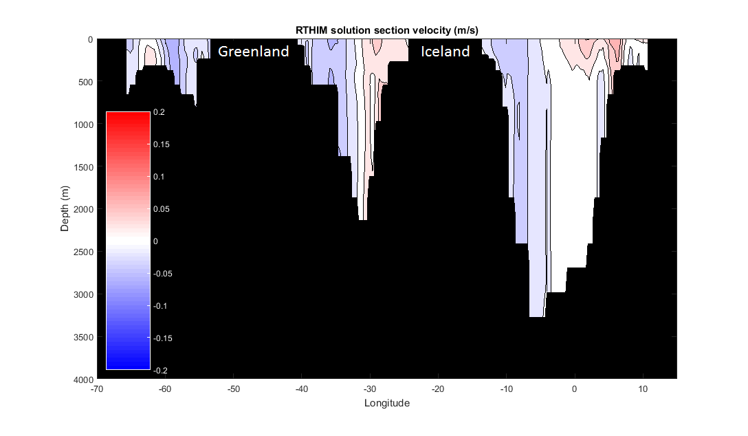
Figure 1: Velocities on the section from an RTHIM solution. The inverse model was applied to the whole of the Arctic, bounded by a line of latitude at 65°N, which is somewhat north of the OSNAP array (only part of the section in longitude is plotted). Red (positive) regions of the plot indicate flow into the Arctic (i.e. northward) and blue (negative) regions indicate flow out of the Arctic (i.e. southward). RTHIM will eventually be applied using a section which coincides with the OSNAP array, to allow a direct comparison with the observations.